13 · Brand lift survey to a brand_funnel model: cost per lifted person

You will learn

• Reweight a brand lift survey for differential non-response
• Correct many lift tests at once with Benjamini-Hochberg
• Turn lift points into people lifted per dollar
• Keep a class E survey out of sales calibration

You need

• Python 3.12 and uv

Run this notebook Offline

notebooks/13_brand_lift_to_brand_funnel.ipynb

Runs offline on your laptop. The outputs on this page were saved from a real run.

About 25 minutes

Access needed. The packages and notebooks are not yet publicly distributed. The steps below need a checkout of the UMP repository. Pages show recorded outputs, so you can follow along without running them.

cd notebooks && uv run jupyter lab

Runs offline. Uses babelfin (import babelfin as fin), plus NumPy, pandas, SciPy and scikit-learn.

Northwind Outdoor’s YouTube video ran for six weeks against 18-34s. The platform’s brand-lift survey came back with +4.2 points of aided awareness. Maya Chen’s first thought: feed it into the sales MMM as a calibration point before Thursday’s budget lock.

UMP says no to that, and then three more snags turn up. This notebook walks through them:

1. a brand-lift survey is class E evidence, so it never calibrates sales incrementality;
2. the survey asked five questions in three age bands, which makes 15 tests and no multiplicity correction;
3. fewer people answered in control, and the ones who did were not like the rest;
4. points of lift are not what a planner buys. People lifted per dollar is, and §25.10 has rules for it.

The answer lands in a brand_funnel model and a benchmark row that stays with Northwind.

In [1]:

import math

import babelfin as fin
import matplotlib.pyplot as plt
import numpy as np
import pandas as pd
from scipy.stats import norm
from sklearn.linear_model import LogisticRegression

pd.set_option("display.max_colwidth", None)
SEED = 7

1. +4.2 points and the urge to calibrate the sales MMM with it

The registry has a brand question: E-BM-BRAND-CPLP, aided awareness people per dollar. A points lift is the same thing before the money: people lifted per 100 exposed people. Babelfin has no keyword for that unit, so we edit the estimand’s dict and wrap it again (the metric_family rides along).

In [2]:

brand = fin.estimand("E-BM-BRAND-CPLP", channels="youtube", weeks=6)


def per_100_exposed(e):
    """The same question, counted per 100 exposed respondents (a points lift)."""
    d = e.to_dict()
    # spec §5: per is spend, impression or absolute, so the denominator goes in the KPI name
    d["unit"] = {"kpi": d["unit"]["kpi"] + "_per_100_exposed_respondents", "per": "absolute",
                 **({"cost_basis": d["unit"]["cost_basis"]} if "cost_basis" in d["unit"] else {})}
    return fin.estimand(d)


aware_pts = per_100_exposed(brand)
headline = fin.number(4.2, (1.9, 6.5), aware_pts, label="Platform headline: YouTube aided awareness lift, 18-34")
print(aware_pts.words, "| family:", aware_pts.spec.metric_family)
headline

Out [2]:

aided awareness people per 100 exposed respondents in total, net from removing all spend, exposed, versus the control counterfactual, over 6 weeks, estimator point, 95% confidence | family: brand_awareness

Platform headline: YouTube aided awareness lift, 18-34: 4.20

likely between 1.90 and 6.50 · low confidence

details

means	aided awareness people per 100 exposed respondents in total, net from removing all spend, exposed, versus the control counterfactual, over 6 weeks, estimator point, 95% confidence
interval	95% confidence 1.90 to 6.50
trust level	2

Maya’s plan was to hand this to the sales MMM. Hold that thought until section 7: the gates will answer it. First, she pulls the respondent-level file and checks the number herself.

2. Survey simulation with differential non-response

A randomised exposed/control survey. Everyone invited is known to the platform, including one covariate: whether they follow outdoor channels (enthusiast). Enthusiasts are more aware of Northwind to begin with, and in control they are also far more willing to answer a survey about it.

Why it matters: a common secondary-source rule of thumb is about 2,000 responses per metric for one headline read. Fifteen cuts need more, so the panel here is larger (about 34,000 responses).

In [3]:

BANDS = ["18_24", "25_34", "35_plus"]
METRICS = ["awareness", "recall", "consideration", "favorability", "intent"]
TRUE = {
    "pp_lift": {
        "awareness": {"18_24": 4.0, "25_34": 5.0, "35_plus": 0.0},
        "consideration": {"18_24": 1.5, "25_34": 2.0, "35_plus": 0.0},
        "recall": {"18_24": 3.0, "25_34": 3.0, "35_plus": 0.0},
        "favorability": dict.fromkeys(BANDS, 0.0),
        "intent": dict.fromkeys(BANDS, 0.0),
    },
    "resp_rate_exposed": 0.12, "resp_rate_control": 0.09,
    "exposed_reach": {"18_24": 640_000, "25_34": 620_000, "35_plus": 140_000},  # 1.4M in total
    "spend": 210_000,
}
TRUE["people_lifted_per_$_awareness_true"] = sum(
    TRUE["pp_lift"]["awareness"][b] / 100 * TRUE["exposed_reach"][b] for b in BANDS) / TRUE["spend"]

BASE = {"awareness": (0.25, 0.55), "recall": (0.10, 0.18), "consideration": (0.05, 0.14),
        "favorability": (0.30, 0.60), "intent": (0.04, 0.12)}          # (non-enthusiast, enthusiast)
RESPONSE = {"exposed": (0.11, 0.14), "control": (0.07, 0.137)}       # gives about 12% and 9% overall
INVITED = {"18_24": 70_000, "25_34": 70_000, "35_plus": 40_000}      # per arm


def simulate(seed):
    rng = np.random.default_rng(seed)
    parts = []
    for arm in ("exposed", "control"):
        for b in BANDS:
            n = INVITED[b]
            enth = rng.random(n) < 0.30
            d = pd.DataFrame({"arm": arm, "band": b, "enthusiast": enth.astype(int)})
            d["responded"] = (rng.random(n) < np.where(enth, RESPONSE[arm][1], RESPONSE[arm][0])).astype(int)
            for m in METRICS:
                p = np.where(enth, BASE[m][1], BASE[m][0]) + (TRUE["pp_lift"][m][b] / 100 if arm == "exposed" else 0)
                d[m] = (rng.random(n) < p).astype(int)
            parts.append(d)
    return pd.concat(parts, ignore_index=True)


invited = simulate(SEED)
invited.groupby("arm").agg(invited=("responded", "size"), response_rate=("responded", "mean")).round(3)

Out [3]:

	invited	response_rate
arm
control	180000	0.090
exposed	180000	0.118

The setback. Among people who answered, control is much heavier on enthusiasts, so control looks more aware than it should.

In [4]:

resp = invited[invited.responded == 1]
resp.groupby("arm").agg(responses=("enthusiast", "size"), enthusiast_share=("enthusiast", "mean")).round(3)

Out [4]:

	responses	enthusiast_share
arm
control	16177	0.464
exposed	21296	0.354

3. Lift per metric and age band; reweighting for non-response

Absolute lift in points is exposed share minus control share, with a two-proportion z interval. The reweighted version models the chance each invited person answered (logistic regression on arm, band and enthusiast) and weights respondents by one over it. The SE uses Kish’s effective sample size.

Assumed: response depends only on what we observed (missing at random given these covariates). The SE ignores the uncertainty in the fitted propensities.

In [5]:

def add_weights(inv):
    exp = (inv.arm == "exposed").astype(float)
    X = pd.get_dummies(inv["band"]).astype(float)
    X["enthusiast"], X["exposed"] = inv.enthusiast, exp
    X["enth_x_exposed"] = inv.enthusiast * exp
    for b in BANDS:
        X[f"exposed_x_{b}"] = exp * (inv.band == b)
    p = LogisticRegression(C=1e6, max_iter=2000).fit(X, inv.responded).predict_proba(X)[:, 1]
    return inv.assign(w=1 / p)


def share(s, col, weighted):
    w = s.w.to_numpy() if weighted else np.ones(len(s))
    p = np.average(s[col], weights=w)
    return p, p * (1 - p) / (w.sum() ** 2 / (w**2).sum())


def lift_table(inv):
    r = add_weights(inv).query("responded == 1")
    rows = []
    for m in METRICS:
        for b in BANDS:
            row = {"metric": m, "band": b, "true_pts": TRUE["pp_lift"][m][b]}
            for tag, weighted in (("unweighted", False), ("reweighted", True)):
                (pe, ve), (pc, vc) = (share(r[(r.arm == a) & (r.band == b)], m, weighted) for a in ("exposed", "control"))
                row[f"{tag}_pts"], row[f"{tag}_se"] = 100 * (pe - pc), 100 * math.sqrt(ve + vc)
            rows.append(row)
    t = pd.DataFrame(rows)
    t["lo"], t["hi"] = t.reweighted_pts - 1.96 * t.reweighted_se, t.reweighted_pts + 1.96 * t.reweighted_se
    t["covers_true"] = t.lo.le(t.true_pts) & t.hi.ge(t.true_pts)
    t["p_value"] = 2 * norm.sf((t.reweighted_pts / t.reweighted_se).abs())
    return t


lift = lift_table(invited)
print("Each number:", aware_pts.words.replace("aided awareness ", "<metric> "))
lift.round(2)

Out [5]:

Each number: <metric> people per 100 exposed respondents in total, net from removing all spend, exposed, versus the control counterfactual, over 6 weeks, estimator point, 95% confidence

	metric	band	true_pts	unweighted_pts	unweighted_se	reweighted_pts	reweighted_se	lo	hi	covers_true	p_value
0	awareness	18_24	4.0	-0.47	0.82	2.81	0.83	1.18	4.44	True	0.00
1	awareness	25_34	5.0	1.80	0.82	5.26	0.83	3.64	6.88	True	0.00
2	awareness	35_plus	0.0	-3.01	1.07	-0.04	1.08	-2.16	2.09	True	0.97
3	recall	18_24	3.0	1.28	0.59	2.16	0.60	0.99	3.32	True	0.00
4	recall	25_34	3.0	2.54	0.60	3.35	0.60	2.18	4.53	True	0.00
5	recall	35_plus	0.0	-0.40	0.76	0.61	0.76	-0.87	2.09	True	0.42
6	consideration	18_24	1.5	0.61	0.48	1.48	0.47	0.55	2.41	True	0.00
7	consideration	25_34	2.0	1.53	0.49	2.41	0.48	1.47	3.35	True	0.00
8	consideration	35_plus	0.0	-0.38	0.62	0.46	0.61	-0.74	1.65	True	0.45
9	favorability	18_24	0.0	-2.32	0.82	0.92	0.84	-0.73	2.57	True	0.27
10	favorability	25_34	0.0	-2.34	0.83	1.11	0.84	-0.54	2.76	True	0.19
11	favorability	35_plus	0.0	-2.24	1.10	1.23	1.12	-0.96	3.42	True	0.27
12	intent	18_24	0.0	-1.30	0.42	-0.37	0.41	-1.17	0.42	True	0.36
13	intent	25_34	0.0	-0.40	0.43	0.48	0.42	-0.34	1.31	True	0.25
14	intent	35_plus	0.0	-0.45	0.58	0.36	0.56	-0.74	1.46	True	0.53

Unweighted, every metric reads low, and the null ones read negative. That is the control group’s extra enthusiasts. Reweighting moves each estimate back toward the truth.

In [6]:

aw = lift[lift.metric.isin(["awareness", "consideration"])].reset_index(drop=True)
y = np.arange(len(aw))
fig, ax = plt.subplots(figsize=(7, 3.6))
ax.errorbar(aw.unweighted_pts, y + 0.15, xerr=1.96 * aw.unweighted_se, fmt="o", color="0.6", label="unweighted")
ax.errorbar(aw.reweighted_pts, y - 0.15, xerr=1.96 * aw.reweighted_se, fmt="o", color="C0", label="reweighted (95%)")
ax.scatter(aw.true_pts, y, marker="x", color="C3", zorder=3, label="truth")
ax.axvline(0, color="0.8", lw=1)
ax.set_yticks(y, aw.metric + " " + aw.band)
ax.set_xlabel("lift, points (people lifted per 100 exposed)")
ax.legend(loc="lower right", fontsize=8)
ax.set_title("YouTube, 6 weeks: awareness and consideration lift")
plt.tight_layout()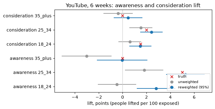

Out [6]:

The campaign bought 18-34. Weighting the two bands by exposed reach gives a figure to set beside the platform’s headline.

In [7]:

def reach_weighted(t, metric, bands, tag="reweighted"):
    s = t[(t.metric == metric) & t.band.isin(bands)].set_index("band")
    w = pd.Series({b: TRUE["exposed_reach"][b] for b in bands})
    w = w / w.sum()
    return float((w * s[f"{tag}_pts"]).sum()), float(math.sqrt(((w * s[f"{tag}_se"]) ** 2).sum()))


v, se = reach_weighted(lift, "awareness", ["18_24", "25_34"])
v_raw, _ = reach_weighted(lift, "awareness", ["18_24", "25_34"], tag="unweighted")
aware_1834 = fin.number(v, (v - 1.96 * se, v + 1.96 * se), aware_pts,
                        label="Reweighted YouTube aided awareness lift, 18-34")
print(f"unweighted 18-34 point: {v_raw:.2f} pts (biased low by non-response); true 18-34: "
      f"{(4.0 * 640 + 5.0 * 620) / 1260:.2f} pts")
aware_1834

Out [7]:

unweighted 18-34 point: 0.65 pts (biased low by non-response); true 18-34: 4.49 pts

Reweighted YouTube aided awareness lift, 18-34: 4.02

likely between 2.87 and 5.17 · medium confidence

details

means	aided awareness people per 100 exposed respondents in total, net from removing all spend, exposed, versus the control counterfactual, over 6 weeks, estimator point, 95% confidence
interval	95% confidence 2.87 to 5.17
trust level	2

4. Fifteen tests, one correction: Benjamini-Hochberg

Five metrics times three bands is 15 tests. At 5% each, about one null would look real by luck alone. BH keeps the false discovery rate at 5% (it holds under the positive dependence of questions answered by the same people).

In [8]:

Q = 0.05


def bh_keep(p, q=Q):
    order = np.argsort(p)
    passed = np.asarray(p)[order] <= q * np.arange(1, len(p) + 1) / len(p)
    k = passed.nonzero()[0].max() + 1 if passed.any() else 0
    keep = np.zeros(len(p), bool)
    keep[order[:k]] = True
    return keep


lift["raw_p_below_5pct"] = lift.p_value < 0.05
lift["bh_keep"] = bh_keep(lift.p_value.to_numpy())
kept = set(zip(lift[lift.bh_keep].metric, lift[lift.bh_keep].band))
lift[["metric", "band", "reweighted_pts", "lo", "hi", "true_pts", "p_value", "raw_p_below_5pct", "bh_keep"]].round(4)

Out [8]:

	metric	band	reweighted_pts	lo	hi	true_pts	p_value	raw_p_below_5pct	bh_keep
0	awareness	18_24	2.8112	1.1845	4.4378	4.0	0.0007	True	True
1	awareness	25_34	5.2632	3.6434	6.8829	5.0	0.0000	True	True
2	awareness	35_plus	-0.0374	-2.1601	2.0853	0.0	0.9725	False	False
3	recall	18_24	2.1556	0.9882	3.3230	3.0	0.0003	True	True
4	recall	25_34	3.3508	2.1755	4.5261	3.0	0.0000	True	True
5	recall	35_plus	0.6101	-0.8707	2.0909	0.0	0.4194	False	False
6	consideration	18_24	1.4815	0.5513	2.4117	1.5	0.0018	True	True
7	consideration	25_34	2.4076	1.4695	3.3457	2.0	0.0000	True	True
8	consideration	35_plus	0.4559	-0.7400	1.6519	0.0	0.4549	False	False
9	favorability	18_24	0.9215	-0.7250	2.5681	0.0	0.2727	False	False
10	favorability	25_34	1.1102	-0.5404	2.7608	0.0	0.1874	False	False
11	favorability	35_plus	1.2267	-0.9627	3.4161	0.0	0.2721	False	False
12	intent	18_24	-0.3747	-1.1735	0.4241	0.0	0.3579	False	False
13	intent	25_34	0.4842	-0.3404	1.3088	0.0	0.2498	False	False
14	intent	35_plus	0.3559	-0.7450	1.4568	0.0	0.5263	False	False

BH keeps awareness, recall and consideration for 18-34 and drops every null. Honest caveat: consideration’s 1.5 to 2 points sit near the edge of what this survey can see. Rerunning the same design with other seeds shows how often BH gets this exact answer.

In [9]:

need = {("awareness", "18_24"), ("awareness", "25_34"), ("consideration", "18_24"), ("consideration", "25_34")}
reruns = []
for s in range(100, 112):
    t = lift_table(simulate(s))
    t["bh_keep"] = bh_keep(t.p_value.to_numpy())
    got = set(zip(t[t.bh_keep].metric, t[t.bh_keep].band))
    reruns.append({"seed": s, "keeps_all_four": need <= got, "null_kept": bool((t.bh_keep & t.true_pts.eq(0)).any())})
reruns = pd.DataFrame(reruns)
print(f"BH kept all four awareness and consideration cells in {reruns.keeps_all_four.mean():.0%} of 12 reruns;"
      f" a null slipped through in {reruns.null_kept.mean():.0%}.")

Out [9]:

BH kept all four awareness and consideration cells in 75% of 12 reruns; a null slipped through in 8%.

5. From points to people per dollar (§25.10)

The conversion: people lifted = points lift / 100 × exposed reach, summed over bands; people per dollar = people lifted / spend. The interval comes from the band SEs (independent arms and bands), carried to the log scale.

One wording. This notebook reports people per dollar, the registry unit (higher is better). §25.10’s cost per person lifted is its reciprocal: dollars per person. Its interval is the reciprocal one, 1/hi to 1/lo.

Platform offset (proposed). §25.10 marks platform-run studies as self-measured: +0.25 on log cost per person lifted (so −0.25 on log people per dollar) and SE × 1.3. Both are placeholders until paired studies estimate them.

In [10]:

OFFSET, SE_INFLATE = 0.25, 1.3   # proposed (spec §25.10 placeholders)


def people_per_dollar(t, metric):
    s = t[t.metric == metric].set_index("band")
    reach, spend = pd.Series(TRUE["exposed_reach"]), TRUE["spend"]
    value = float((s.reweighted_pts / 100 * reach).sum() / spend)
    se = float(math.sqrt(((s.reweighted_se / 100 * reach) ** 2).sum()) / spend)
    return value, se / value                     # value, SE on the log scale (delta method)


def log_interval(log_v, log_se):
    return math.exp(log_v - 1.96 * log_se), math.exp(log_v + 1.96 * log_se)


consid = fin.estimand("E-BM-BRAND-CPLP-CONSID", channels="youtube", weeks=6)
v, lse = people_per_dollar(lift, "awareness")
ppd = fin.number(v, log_interval(math.log(v), lse), brand, label="YouTube aided awareness people per dollar")
ppd_offset = fin.number(math.exp(math.log(v) - OFFSET), log_interval(math.log(v) - OFFSET, SE_INFLATE * lse), brand,
                        label="YouTube aided awareness people per dollar, platform offset (proposed)")
cv, clse = people_per_dollar(lift, "consideration")
ppd_consid_offset = fin.number(math.exp(math.log(cv) - OFFSET), log_interval(math.log(cv) - OFFSET, SE_INFLATE * clse),
                               consid, label="YouTube consideration people per dollar, platform offset (proposed)")
TRUE_PPD = TRUE["people_lifted_per_$_awareness_true"]
TRUE_PPD_CONSID = sum(TRUE["pp_lift"]["consideration"][b] / 100 * TRUE["exposed_reach"][b] for b in BANDS) / TRUE["spend"]

pd.DataFrame([{"number": n.label, "value": n.value, "lo": n.lo, "hi": n.hi, "truth": tv,
               "covers_truth": n.lo <= tv <= n.hi,
               "$ per person lifted": 1 / n.value, "$ lo": 1 / n.hi, "$ hi": 1 / n.lo,
               "estimand": n.estimand.words}
              for n, tv in ((ppd, TRUE_PPD), (ppd_offset, TRUE_PPD), (ppd_consid_offset, TRUE_PPD_CONSID))]).round(3)

Out [10]:

	number	value	lo	hi	truth	covers_truth	$ per person lifted	$ lo	$ hi	estimand
0	YouTube aided awareness people per dollar	0.241	0.180	0.322	0.270	True	4.153	3.101	5.561	aided awareness people per dollar, net from removing all spend, exposed, versus the control counterfactual, over 6 weeks, estimator point, 95% confidence
1	YouTube aided awareness people per dollar, platform offset (proposed)	0.188	0.128	0.274	0.270	True	5.332	3.648	7.794	aided awareness people per dollar, net from removing all spend, exposed, versus the control counterfactual, over 6 weeks, estimator point, 95% confidence
2	YouTube consideration people per dollar, platform offset (proposed)	0.093	0.060	0.144	0.105	True	10.766	6.929	16.727	consideration people per dollar, net from removing all spend, exposed, versus the control counterfactual, over 6 weeks, estimator point, 95% confidence

Before the offset the interval covers the truth (0.27). The offset pulls the point down and widens the band; here it still just covers. The truth in this simulation has no platform bias, so the offset is pure caution. On a real platform study nobody knows that, which is why the offset exists.

In [11]:

ppd_offset

Out [11]:

YouTube aided awareness people per dollar, platform offset (proposed): 0.19

likely between 0.13 and 0.27 · low confidence

details

means	aided awareness people per dollar, net from removing all spend, exposed, versus the control counterfactual, over 6 weeks, estimator point, 95% confidence
interval	95% confidence 0.13 to 0.27
trust level	2

6. Estimands for brand numbers: fin.compare across weeks and against ROI

An older four-week YouTube study answers almost the same question. A sales ROI answers a different one.

In [12]:

brand_4wk = fin.estimand("E-BM-BRAND-CPLP", channels="youtube", weeks=4)
pd.DataFrame([{"pair": name, "rung": a.rung, "combinable": a.combinable, "differs on": ", ".join(a.mismatched)}
              for name, a in (("6 weeks vs 4 weeks", fin.compare(brand, brand_4wk)),
                              ("awareness vs consideration", fin.compare(brand, consid)),
                              ("awareness vs sales ROI", fin.compare(brand, fin.estimand("roi"))))])

Out [12]:

	pair	rung	combinable	differs on
0	6 weeks vs 4 weeks	assumed_alignment	True	horizon
1	awareness vs consideration	side_by_side	False	unit
2	awareness vs sales ROI	side_by_side	False	intervention, baseline, horizon, unit, point_rule, interval, applies_to

Six weeks against four is assumed_alignment: usable, with the assumption labelled and the interval widened. Against ROI it is side_by_side: shown together, never combined.

7. Class E TestResult: excluded from sales calibration

Back to Maya’s first plan. Babelfin has no TestResult wrapper, so this is a plain dict checked with fin.check(..., operation="calibrate").

In [13]:

test_doc = {"channel": "youtube", "admissibility_class": "E", "method": "platform_reported", "estimand": brand.to_dict(),
            "lift": fin.number(4.2, (1.9, 6.5), brand).to_dict(), "outcome": "positive", "duration_weeks": 6,
            "provenance_tier": "platform-reported", "applies_to": {"media_ids": ["youtube"]}}
fin.validate("test_result", test_doc)
report_calibrate = fin.check("test_result", test_doc, operation="calibrate")
report_calibrate.to_frame()

Out [13]:

	gate	outcome	message	codes
0	G-EXP-01	fallback	not pre-registered	NOT_PREREGISTERED

G-EXP-05 excludes it and the run continues: survey brand lift never calibrates sales incrementality. G-EXP-01 adds that the study was not pre-registered.

For brand use, the result says which family it belongs to. Note: the gate reads a top-level metric_family key on the result, not the one inside the estimand.

In [14]:

report_brand = fin.check("test_result", {**test_doc, "metric_family": "brand_awareness"}, operation="calibrate")
report_brand.to_frame()

Out [14]:

	gate	outcome	message	codes
0	G-EXP-01	fallback	not pre-registered	NOT_PREREGISTERED

8. brand_funnel Tier D manifest and m.check()

First the funnel: how much of the awareness lift carried down to consideration, per band (reweighted points).

In [15]:

pts = lift.set_index(["metric", "band"])
rows = []
for b in ["18_24", "25_34"]:
    a, sa = pts.loc[("awareness", b), ["reweighted_pts", "reweighted_se"]]
    c, sc = pts.loc[("consideration", b), ["reweighted_pts", "reweighted_se"]]
    r = c / a
    se = abs(r) * math.sqrt((sc / c) ** 2 + (sa / a) ** 2)   # delta method, covariance set to 0 (assumed)
    rows.append({"band": b, "awareness": a, "consideration": c, "consideration_per_aware": r,
                 "lo": r - 1.96 * se, "hi": r + 1.96 * se,
                 "true_ratio": TRUE["pp_lift"]["consideration"][b] / TRUE["pp_lift"]["awareness"][b]})
funnel = pd.DataFrame(rows).set_index("band")
funnel["covers_truth"] = funnel.lo.le(funnel.true_ratio) & funnel.hi.ge(funnel.true_ratio)
print("Lifts in", aware_pts.words.replace("aided awareness ", "<metric> "))
print("Ratio: consideration points per awareness point, same band, 95% interval (delta method)")
funnel.round(2)

Out [15]:

Lifts in <metric> people per 100 exposed respondents in total, net from removing all spend, exposed, versus the control counterfactual, over 6 weeks, estimator point, 95% confidence
Ratio: consideration points per awareness point, same band, 95% interval (delta method)

	awareness	consideration	consideration_per_aware	lo	hi	true_ratio	covers_truth
band
18_24	2.81	1.48	0.53	0.08	0.98	0.38	True
25_34	5.26	2.41	0.46	0.23	0.68	0.40	True

The ratio of two noisy lifts is noisier still. For 18 to 24 it runs 0.08 to 0.98; for 25 to 34, 0.23 to 0.68. Both cover the truth (0.38, 0.40). Read it as a range, not a rate.

Why the covariance is set to 0. Both lifts come from the same respondents, so they likely move together. A positive covariance shrinks the ratio’s variance, so dropping it makes the interval wider: an assumption, labelled, on the cautious side.

Tier D summaries only take metric="roi" or "mroi", so the brand number sits under the roi label and the estimand carries what it means. Meta’s figure is an illustrative one from a Q2 study on file, not re-analysed here. Consideration goes in notes.

In [16]:

meta_ppd = fin.number(0.19, (0.12, 0.29), brand, label="Meta aided awareness people per dollar (Q2 study, on file)")
m = fin.Model.from_table(
    {"youtube": ppd_offset, "meta": meta_ppd},
    estimand=fin.estimand("E-BM-BRAND-CPLP", weeks=6), name="northwind_brand_funnel", engine="survey-funnel",
    family="brand_funnel", metric="roi", dependence="declared_assumption",
    notes=[{"code": "FUNNEL_CONSIDERATION", "estimand_id": "E-BM-BRAND-CPLP-CONSID",
            "youtube": ppd_consid_offset.to_dict()},
           {"code": "PLATFORM_OFFSET_PROPOSED", "log_offset": OFFSET, "se_multiplier": SE_INFLATE}],
)
model_report = m.check()
print(m, "|", model_report.next_state)
model_report.to_frame()

Out [16]:

<Model 'northwind_brand_funnel' Tier D, 2 channels> | checks_passed

	gate	outcome	message	codes
0	G-ACC-01	fallback	acceptance untested: usable, labelled unvalidated method, trust reduced	UNVALIDATED_METHOD
1	G-CAP-01	route	sandbox output: experimental label and a named approver needed	EXPERIMENTAL_LABEL

Two labels, no stops. G-ACC-01: no acceptance run yet, so trust is reduced. G-CAP-01: a sandbox model needs the experimental label and a named approver. Gap: no gate checks the §16 brand family bar (recovery, nulls); this notebook’s truth checks stand in for it.

9. A benchmark row that stays client_only

The row stores log cost per person lifted (the benchmark convention), so the sign flips: offset +0.25 and SE × 1.3. Babelfin has no wrapper; the typed model is ump_spec.models.BenchmarkEvidence and the kind is benchmark_row. The study’s licence is client-only.

In [17]:

row = {"client_ref": "c_7f31a", "channel": "youtube", "vertical": "outdoor_retail", "quarter": "2026 Q3",
       "source_type": "brand_lift_platform", "estimand_id": "E-BM-BRAND-CPLP", "admissibility_class": "E",
       "log_value": -math.log(ppd.value) + OFFSET, "se": SE_INFLATE * lse,
       "metric_family": "brand_awareness", "licence": "client_only", "spend": float(TRUE["spend"]),
       "moderators": {"self_measured": True}, "notes": ["PLATFORM_OFFSET_PROPOSED"]}
fin.validate("benchmark_row", row)
bm_report = fin.check("benchmark_row", row)
bm_report.to_frame()

Out [17]:

	gate	outcome	message	codes
0	G-BM-07	exclude_and_continue	held from pool: missing ['confidence_level', 'value_basis']	HELD_FROM_POOL
1	G-BM-09	fallback	licence client-only: kept out of pooled cells	LICENSE_CLIENT_ONLY

G-BM-09 falls back to client_only: it still feeds Northwind’s own plans, never a cross-brand cell. G-BM-07 holds it from the pool for a second reason, a missing level and basis. Adding them clears that one.

In [18]:

bm_report_full = fin.check("benchmark_row", {**row, "confidence_level": 0.95, "value_basis": "net"})
bm_report_full.to_frame()

Out [18]:

	gate	outcome	message	codes
0	G-BM-09	fallback	licence client-only: kept out of pooled cells	LICENSE_CLIENT_ONLY

10. What Maya hands over

• Asked: is the +4.2-point YouTube brand lift worth acting on, and can it calibrate the sales MMM?
• Calibration: no. Class E is excluded from sales calibration (G-EXP-05); it is filed as brand evidence.
• Handed over: below, with its estimand.
• Assumed or fell back: missing at random given arm, band and enthusiast; BH at 5% across 15 tests; the §25.10 platform offset (0.25 log, SE × 1.3) is proposed; the model is Tier D, untested (G-ACC-01), sandbox (G-CAP-01); the benchmark row is client-only.
• Next: buy a 4-week independent panel read (class E, no platform offset) to check the offset, and size the next survey for consideration, which is near the edge of what this one could see.

In [19]:

pd.DataFrame([{"number": n.label, "value": round(n.value, 3), "interval": f"{n.lo:.3f} to {n.hi:.3f}",
               "level": n.level, "estimand": n.estimand.words}
              for n in (aware_1834, ppd, ppd_offset, ppd_consid_offset)])

Out [19]:

	number	value	interval	level	estimand
0	Reweighted YouTube aided awareness lift, 18-34	4.018	2.870 to 5.166	0.95	aided awareness people per 100 exposed respondents in total, net from removing all spend, exposed, versus the control counterfactual, over 6 weeks, estimator point, 95% confidence
1	YouTube aided awareness people per dollar	0.241	0.180 to 0.322	0.95	aided awareness people per dollar, net from removing all spend, exposed, versus the control counterfactual, over 6 weeks, estimator point, 95% confidence
2	YouTube aided awareness people per dollar, platform offset (proposed)	0.188	0.128 to 0.274	0.95	aided awareness people per dollar, net from removing all spend, exposed, versus the control counterfactual, over 6 weeks, estimator point, 95% confidence
3	YouTube consideration people per dollar, platform offset (proposed)	0.093	0.060 to 0.144	0.95	consideration people per dollar, net from removing all spend, exposed, versus the control counterfactual, over 6 weeks, estimator point, 95% confidence

Going deeper

• §25.10 of the spec: metric families, the platform offset and licences. §6 of the spec: admissibility classes.
• ump_spec.models.TestResult, BenchmarkEvidence and ModelManifest hold the full contract.
• The registry titles brand estimands cost per person lifted while the unit reads people per dollar; this notebook uses the unit and gives the reciprocal.

Next: 01 · Estimands and shown numbers for estimands from the start, or 02 · Validate and gate a document offline for more on gates.