12 · Clean-room overlap, deduplicated reach and frequency curves
You will learn
- Work with suppressed, noised clean-room aggregates
- See the privacy hard stops (G-PRIV-01 to 03) fire offline
- Fit beta-binomial reach curves and check them against panel truth
- Combine vehicles without double counting, and declare the duplication assumption
You need
- Python 3.12 and uv
Runs offline. Uses babelfin, NumPy, SciPy and matplotlib. The data is SYNTHETIC, generated below with a known
truth.
Northwind Outdoor sends Sam Patel two questions on a Monday. How many of its 180,000 CRM customers can two partner publishers reach? And what will 400 GRPs across CTV and YouTube buy among adults 25 to 54?
Sam’s first deck went out fast and came back with red ink. It called the 62% match rate “overlap”. It added the two vehicles’ reach with Sainsbury’s independence formula, which overstates combined reach when the same outdoorsy people watch both. And the clean-room totals ran low, because cells under the privacy floor came back blank. This notebook is the second deck.
import hashlib
import babelfin as finimport matplotlib.pyplot as pltimport numpy as npimport pandas as pdfrom scipy.special import expitfrom scipy.stats import betabinom, binom
SEED = 11VEHICLES = ["ctv", "youtube"]COLOURS = {"ctv": "#2a6fdb", "youtube": "#d4572a"}pd.set_option("display.max_colwidth", None)   # an estimand is a sentence; never cut it short

def table(numbers):    """fin.Numbers as rows: value, interval and the estimand in words."""    return pd.DataFrame([{"number": k, "value": round(a.value, 1), "lo": round(a.lo, 1), "hi": round(a.hi, 1),                          "estimand": a.estimand.words} for k, a in numbers.items()]).set_index("number")
1. Two client questions and a deck that mixed match rate with overlap
Section titled “1. Two client questions and a deck that mixed match rate with overlap”Three words did the damage, so pin them down first.
| Word | Means | Northwind’s question |
|---|---|---|
| Match rate | share of CRM customers found at either publisher | “can they reach them at all?” |
| Overlap | share of CRM customers found at both publishers | “how much do the two buys repeat each other?” |
| Deduplicated reach | people reached at least once by either vehicle, counted once | “how many people does the plan touch?” |
The first deck put the match rate in the overlap box and summed the two publishers’ matched counts as if nobody sat in both. Both mistakes push the answer up.
2. A synthetic population with correlated exposure
Section titled “2. A synthetic population with correlated exposure”Two million adults 25 to 54. Each has a latent outdoor interest. Interest raises the chance of holding an
account at each publisher, and it raises how often an account holder sees a spot. The two vehicles’ viewing
propensities share half their variance (interest_corr 0.5), so heavy CTV viewers tend to be heavy YouTube
viewers too. Each insertion delivers about 10 GRPs, so 200 GRPs is 20 spots; a person’s frequency is a binomial
draw on their own per-spot probability, which makes the population frequency a mixture (negative-binomial-like).
TRUE holds what the world was built to have. truth measures this draw exactly, from every person’s probability.
The 3+ target is 0.37: each vehicle alone reaches about 23% at 3+, so the pair cannot reach fewer.
TRUE = {"universe_25_54": 2_000_000, "crm_size": 180_000, "match_rate": 0.62, "crm_overlap_pubA_pubB": 0.27,        "interest_corr": 0.5, "reach1_ctv_200grp": 0.41, "reach1_yt_200grp": 0.36, "combined_reach1_true": 0.52,        "combined_reach1_sainsbury": 0.62, "reach3_combined_true": 0.37, "suppression_k": 50, "dp_epsilon": 1.0}
N, RHO, GRP_PER_SPOT = TRUE["universe_25_54"], TRUE["interest_corr"], 10DESIGN = {"ctv": {"account": 0.68, "per_spot": -3.14}, "youtube": {"account": -0.23, "per_spot": -2.94}}ACCOUNT_LOAD, SPREAD = 2.59, 1.99   # how strongly interest drives accounts, and the spread of per-spot viewing
rng = np.random.default_rng(SEED)interest = rng.normal(size=N)account, p = {}, {}for v, d in DESIGN.items():    account[v] = rng.random(N) < expit(d["account"] + ACCOUNT_LOAD * interest)    own = np.sqrt(RHO) * interest + np.sqrt(1 - RHO) * rng.normal(size=N)    p[v] = account[v] * expit(d["per_spot"] + SPREAD * own)   # per-spot chance of seeing the ad

def spots(grps):    n = np.rint(np.asarray(grps) / GRP_PER_SPOT).astype(int)    return int(n) if n.ndim == 0 else n

def reach_true(v, grps, k=1):    """Expected share of the universe seeing vehicle v at least k times."""    return float(binom.sf(k - 1, spots(grps), p[v]).mean())

def combined_true(grps_each, k=1):    """Expected share seeing at least k spots across both vehicles (each vehicle at grps_each)."""    n = spots(grps_each)    below = sum(binom.pmf(i, n, p["ctv"]) * binom.pmf(j, n, p["youtube"])                for i in range(k) for j in range(k - i))    return float(1 - below.mean())

r_ctv, r_yt = reach_true("ctv", 200), reach_true("youtube", 200)truth = {"reach1_ctv_200grp": r_ctv, "reach1_yt_200grp": r_yt, "combined_reach1_true": combined_true(200), "combined_reach1_sainsbury": 1 - (1 - r_ctv) * (1 - r_yt), "reach3_combined_true": combined_true(200, k=3)}pd.DataFrame({"built to (TRUE)": {k: TRUE[k] for k in truth}, "this draw": truth}).round(3)| built to (TRUE) | this draw | |
|---|---|---|
| reach1_ctv_200grp | 0.41 | 0.410 |
| reach1_yt_200grp | 0.36 | 0.361 |
| combined_reach1_true | 0.52 | 0.520 |
| combined_reach1_sainsbury | 0.62 | 0.622 |
| reach3_combined_true | 0.37 | 0.370 |
Already the trap is visible: Sainsbury’s formula, applied to the true single-vehicle reaches, says about 62%. The true combined reach is about 52%. Ten points of the plan’s headline come from assuming the two audiences are strangers.
3. The clean-room join: aggregates only, suppressed and noised
Section titled “3. The clean-room join: aggregates only, suppressed and noised”Northwind uploads hashed emails. Each publisher matches them against its own hashed IDs, and the campaign’s exposure logs ride along inside the clean room. Nothing member-level leaves. What comes back:
- cells (60 regions x 3 age bands), each count blank when it is below k = 50 (proposed, illustrative);
- Laplace noise on every released count, scale 1/ε with ε = 1.0 per count (proposed, illustrative);
- a query budget; each release spends one, and every release first passes the privacy gates.
The CleanRoom class below is a stand-in for the partner’s room. Its _release runs fin.check on the clean-room
dataset with the destination, the cell sizes, the aggregate and the remaining budget, so G-PRIV-01 to G-PRIV-03 decide
what leaves. A release that leaves any of them out fails closed.
crm_rng = np.random.default_rng(SEED + 1)# CRM customers lean slightly outdoorsy: a weighted draw without replacement (Gumbel top-k).keys = 0.1 * interest + crm_rng.gumbel(size=N)crm = np.argpartition(-keys, TRUE["crm_size"])[:TRUE["crm_size"]]HASH_MATCH = 0.80 # a hashed email finds its account 80% of the timeregions = np.array([f"R{i:02d}" for i in range(1, 61)])region_w = 1 / np.arange(1, 61) ** 1.2rows = pd.DataFrame({ "region": crm_rng.choice(regions, len(crm), p=region_w / region_w.sum()), "age_band": crm_rng.choice(["25-34", "35-44", "45-54"], len(crm), p=[0.35, 0.33, 0.32]),})for v, tag in [("ctv", "a"), ("youtube", "b")]: matched = account[v][crm] & (crm_rng.random(len(crm)) < HASH_MATCH) freq = crm_rng.binomial(spots(200), p[v][crm]) * matched # exposure is only visible for matched IDs rows[f"matched_{tag}"], rows[f"freq_{tag}"] = matched.astype(int), freqrows["matched_both"] = rows.matched_a & rows.matched_brows["matched_either"] = rows.matched_a | rows.matched_brows["seen_a"], rows["seen_b"] = (rows.freq_a > 0).astype(int), (rows.freq_b > 0).astype(int)rows["seen_both"] = rows.seen_a & rows.seen_brows["seen_3plus"] = ((rows.freq_a + rows.freq_b) >= 3).astype(int)for tag in "ab": for f in (1, 2): rows[f"{tag}_f{f}"] = (rows[f"freq_{tag}"] == f).astype(int)rows["rows"] = 1print(f"{len(rows):,} CRM rows; they stay inside the clean room")180,000 CRM rows; they stay inside the clean room
K, EPSILON = TRUE["suppression_k"], TRUE["dp_epsilon"]

def dup_factor(t):    """P(seen by both) / (P(seen by ctv) * P(seen by youtube)): 1.0 is independence."""    return (t["seen_both"] / t["rows"]) / ((t["seen_a"] / t["rows"]) * (t["seen_b"] / t["rows"]))
_h = hashlib.sha256(b"northwind-pubA-pubB-clean-room-overlap").hexdigest()CR_DOC = {"ref": f"dataset://northwind-outdoor/cleanroom_overlap@sha256:{_h}", "scope": "northwind-outdoor",          "name": "cleanroom_overlap", "sha256": _h, "client_id": "northwind-outdoor",          "delivery": {"source": "clean room: publisher A (CTV) x publisher B (online video)", "file_fingerprint": _h}}

class CleanRoom:    """Stand-in for a partner clean room. Member rows never leave; aggregates leave after the privacy gates."""
    def __init__(self, rows, *, k, epsilon, budget, seed):        self._rows, self.k, self.epsilon, self.budget = rows, k, epsilon, budget        self.released, self._rng = [], np.random.default_rng(seed)
    def _release(self, aggregates, segments=None):        # Aggregates go to Northwind (the client). A total has no cells, so its own count is its segment size.        if segments is None:            segments = [{"id": a["query"], "size": a["n"]} for a in aggregates]        ctx = {"destination": "client", "segments": segments,               "released_aggregates": self.released, "query_budget_remaining": self.budget}        for agg in aggregates:           # every aggregate is checked against what already left            fin.check("dataset", CR_DOC, operation="release", context={**ctx, "aggregate": agg}).raise_for_stops()        self.released += aggregates        self.budget -= 1
    def _noise(self, n):        return n + self._rng.laplace(0, 1 / self.epsilon, size=np.shape(n))
    def cells(self, metrics, by=("region", "age_band"), suppress=True):        true = self._rows.groupby(list(by))[metrics].sum()        shown = true.where(true >= self.k) if suppress else true        segments = [{"id": f"{'|'.join(i)}|{m}", "size": int(shown.loc[i, m])}                    for i in shown.index for m in metrics if pd.notna(shown.loc[i, m])]        aggs = [{"query": f"select {', '.join(by)}, sum({m}) from crm_join group by {', '.join(by)}",                 "n": int(shown[m].sum())} for m in metrics]        self._release(aggs, segments)        return self._noise(shown).round()
    def totals(self, metrics):        true = self._rows[metrics].sum()        self._release([{"query": f"select sum({m}) from crm_join", "n": int(true[m])} for m in metrics])        return self._noise(true.astype(float)).round()

room = CleanRoom(rows, k=K, epsilon=EPSILON, budget=3, seed=SEED + 2)
The cell table, and why its total runs low
Section titled “The cell table, and why its total runs low”The first query asks for every count by region and age band. Small regions produce cells under k; those come back blank.
METRICS = ["matched_a", "matched_b", "matched_both", "matched_either", "seen_a", "seen_b", "seen_both", "seen_3plus", "a_f1", "a_f2", "b_f1", "b_f2"]cell_table = room.cells(METRICS)suppressed = cell_table.isna().sum()naive = cell_table.sum()pd.DataFrame({"cells blank (< k)": suppressed, "sum of visible cells": naive}).loc[ ["matched_either", "matched_both", "seen_both", "seen_3plus"]].astype(int)| cells blank (< k) | sum of visible cells | |
|---|---|---|
| matched_either | 0 | 112361 |
| matched_both | 47 | 47204 |
| seen_both | 83 | 29267 |
| seen_3plus | 19 | 60244 |
Adding up the visible cells is the naive total, and it is biased low by construction: every blank cell holds somewhere between 1 and 49 people. The fix is one more release, the grand totals, which carry no small cells. The difference between the two is the suppressed mass, and it gets disclosed next to the number.
TOTAL_METRICS = ["rows", *METRICS]totals = room.totals(TOTAL_METRICS)dp_half = np.log(1 / 0.10) / EPSILON # 90% half-width of one Laplace countdisclosure = pd.DataFrame({"naive (visible cells)": naive, "grand total (noised)": totals[METRICS], "suppressed mass": totals[METRICS] - naive, "naive shortfall %": 100 * (totals[METRICS] - naive) / totals[METRICS]})print(f"Disclosed: {int(suppressed.sum())} of {cell_table.size} cells blank below k={K} (proposed); Laplace noise " f"eps={EPSILON} per count (proposed), 90% +/-{dp_half:.1f} people per count; budget left {room.budget}")disclosure.loc[["matched_either", "matched_both", "seen_both", "seen_3plus"]].round(1)Disclosed: 764 of 2160 cells blank below k=50 (proposed); Laplace noise eps=1.0 per count (proposed), 90% +/-2.3 people per count; budget left 1
| naive (visible cells) | grand total (noised) | suppressed mass | naive shortfall % | |
|---|---|---|---|---|
| matched_either | 112361.0 | 112370.0 | 9.0 | 0.0 |
| matched_both | 47204.0 | 49112.0 | 1908.0 | 3.9 |
| seen_both | 29267.0 | 31949.0 | 2682.0 | 8.4 |
| seen_3plus | 60244.0 | 61093.0 | 849.0 | 1.4 |
true_counts = rows[METRICS].sum()crm_n = totals["rows"]match_rate, overlap = totals["matched_either"] / crm_n, totals["matched_both"] / crm_nprint(f"match rate {match_rate:.1%} (built {TRUE['match_rate']:.0%}); " f"overlap {overlap:.1%} (built {TRUE['crm_overlap_pubA_pubB']:.0%})")print(f"naive matched_either runs {true_counts['matched_either'] - naive['matched_either']:,.0f} people low; " f"the grand total is off the true count by {totals['matched_either'] - true_counts['matched_either']:+.0f}")print(f"duplication factor from visible cells {dup_factor({**naive, "rows": crm_n}):.2f} vs from grand totals " f"{dup_factor(totals):.2f}")match rate 62.4% (built 62%); overlap 27.3% (built 27%) naive matched_either runs 10 people low; the grand total is off the true count by -1 duplication factor from visible cells 1.52 vs from grand totals 1.61
The headline count barely moves: CRM customers matched at either publisher sit in big cells. The shortfall lands on the rare counts (both publishers, seen twice, seen by both), and those are the counts duplication is built from. Read off the visible cells, the duplication factor comes out too low, and the combined reach in section 6 would drift back toward Sainsbury.
4. Privacy gates in action
Section titled “4. Privacy gates in action”Four requests Sam tried during the week. Each is a hard stop in UMP (Why: privacy is one of the eight stops that
never degrade; on_gate_fail: "strict" changes nothing here).
# (a) Ask for the cells without suppression: the 31-person cells would leave.try: room.cells(["matched_both"], suppress=False)except fin.Stopped as stop: print(stop.code, "|", stop)PRIVACY_FLOOR | PRIVACY_FLOOR: G-PRIV-01: 47 segment(s) below minimum size 50
# (b) A week later ten new customers land in the CRM upload; Sam reruns the same total.late = rows.sample(10, random_state=SEED).assign(region="R60")room._rows = pd.concat([rows, late], ignore_index=True)try: room.totals(["rows"])except fin.Stopped as stop: print(stop.code, "|", stop) print("Why: the two answers differ by exactly ten people, so subtracting them would describe those ten.")room._rows = rowsPRIVACY_FLOOR | PRIVACY_FLOOR: G-PRIV-03: differencing risk: differs from a released aggregate by 10 < 50 Why: the two answers differ by exactly ten people, so subtracting them would describe those ten.
# (c) One last breakdown spends the budget; the next request is refused.by_age = room.cells(["seen_both"], by=("age_band",))print("budget left:", room.budget)try: room.cells(["seen_3plus"], by=("age_band",))except fin.Stopped as stop: print(stop.code, "|", stop)budget left: 0 PRIVACY_FLOOR | PRIVACY_FLOOR: G-PRIV-03: query budget spent
# (d) Copying rows out of an aggregates_only room whose read reports no cell sizes fails closed.read = {"access": {"copy_policy": "aggregates_only"}, "segments": [], # the read came back with no cells "payload": {"columns": list(rows.columns)}, "aggregate": {"query": "select * from crm_join", "n": len(rows)}}report = fin.check("dataset", CR_DOC, operation="materialize", context=read)try: report.raise_for_stops()except fin.Stopped as stop: print(stop.code, "|", stop)report.to_frame()[["gate", "outcome", "message"]]PRIVACY_FLOOR | PRIVACY_FLOOR: G-PRIV-01: aggregates_only read reported no cell sizes; the floor cannot be checked
| gate | outcome | message | |
|---|---|---|---|
| 0 | G-PRIV-01 | hard_stop | aggregates_only read reported no cell sizes; the floor cannot be checked |
5. Per-vehicle reach curves (beta-binomial), checked against panel truth
Section titled “5. Per-vehicle reach curves (beta-binomial), checked against panel truth”Each publisher shares a frequency log from the current flight: 20,000 sampled people in the universe and how many of the 20 spots each saw. The beta-binomial (Metheringham) model says each person has their own per-spot chance, drawn from a Beta(α, β); fit it by the method of moments, then change the number of spots to read reach at other GRP levels. A bootstrap over the log gives the interval.
The check the reach and frequency profile asks for (spec §16) is coverage against panel truth. A separate panel of 5,000 people measured past flights at 50, 100, 200 and 400 GRPs. A level counts as covered when the panel point sits within 1.645 combined standard errors of the curve (curve bootstrap plus panel sampling). UMP runs no gate for this, so it is run here by hand.
LOG_N, PANEL_N, BOOT = 20_000, 5_000, 300LEVELS = [50, 100, 200, 400]fit_rng = np.random.default_rng(SEED + 3)

def bb_mom(x, n):    """Beta-binomial (alpha, beta) by the method of moments from frequencies x out of n spots."""    mu = x.mean() / n    icc = (x.var(ddof=1) / (n * mu * (1 - mu)) - 1) / (n - 1)    ab = (1 - icc) / icc    return mu * ab, (1 - mu) * ab

def bb_reach(alpha, beta, grps, k=1):    return betabinom.sf(k - 1, spots(grps), alpha, beta)

fits, panel = {}, {}for v in VEHICLES:    log = fit_rng.binomial(spots(200), p[v][fit_rng.choice(N, LOG_N, replace=False)])    boot = np.array([bb_mom(fit_rng.choice(log, LOG_N), spots(200)) for _ in range(BOOT)])    fits[v] = {"log": log, "alpha_beta": bb_mom(log, spots(200)), "boot": boot}    who = fit_rng.choice(N, PANEL_N, replace=False)    panel[v] = {g: fit_rng.binomial(spots(g), p[v][who]) for g in LEVELS}
rows_cov = []for v in VEHICLES: a, b = fits[v]["alpha_beta"] for k in (1, 3): for g in LEVELS: draws = bb_reach(fits[v]["boot"][:, 0], fits[v]["boot"][:, 1], g, k) pan = (panel[v][g] >= k).mean() se = np.sqrt(draws.var() + pan * (1 - pan) / PANEL_N) curve = bb_reach(a, b, g, k) rows_cov.append({"vehicle": v, "reach": f"{k}+", "grps": g, "curve %": 100 * curve, "lo %": 100 * np.quantile(draws, 0.05), "hi %": 100 * np.quantile(draws, 0.95), "panel %": 100 * pan, "covered": abs(curve - pan) <= 1.645 * se, "truth %": 100 * reach_true(v, g, k)})coverage = pd.DataFrame(rows_cov)coverage.round(1)| vehicle | reach | grps | curve % | lo % | hi % | panel % | covered | truth % | |
|---|---|---|---|---|---|---|---|---|---|
| 0 | ctv | 1+ | 50 | 25.2 | 24.8 | 25.6 | 25.3 | True | 25.5 |
| 1 | ctv | 1+ | 100 | 32.8 | 32.3 | 33.3 | 33.4 | True | 33.5 |
| 2 | ctv | 1+ | 200 | 40.2 | 39.5 | 40.8 | 40.8 | True | 41.0 |
| 3 | ctv | 1+ | 400 | 47.0 | 46.2 | 47.7 | 48.0 | True | 47.3 |
| 4 | ctv | 3+ | 50 | 7.0 | 6.8 | 7.3 | 6.5 | True | 6.9 |
| 5 | ctv | 3+ | 100 | 15.0 | 14.7 | 15.3 | 13.7 | False | 14.8 |
| 6 | ctv | 3+ | 200 | 23.6 | 23.1 | 24.0 | 22.6 | True | 23.9 |
| 7 | ctv | 3+ | 400 | 32.0 | 31.4 | 32.5 | 33.1 | True | 33.2 |
| 8 | youtube | 1+ | 50 | 23.9 | 23.5 | 24.3 | 24.0 | True | 24.0 |
| 9 | youtube | 1+ | 100 | 30.6 | 30.1 | 31.1 | 30.7 | True | 30.4 |
| 10 | youtube | 1+ | 200 | 37.1 | 36.5 | 37.7 | 36.3 | True | 36.1 |
| 11 | youtube | 1+ | 400 | 43.1 | 42.4 | 43.9 | 41.1 | False | 40.5 |
| 12 | youtube | 3+ | 50 | 7.5 | 7.3 | 7.8 | 7.5 | True | 7.5 |
| 13 | youtube | 3+ | 100 | 14.9 | 14.6 | 15.2 | 15.0 | True | 15.1 |
| 14 | youtube | 3+ | 200 | 22.5 | 22.1 | 22.9 | 23.3 | True | 23.2 |
| 15 | youtube | 3+ | 400 | 29.8 | 29.3 | 30.3 | 31.0 | False | 30.7 |
cov_summary = coverage.groupby(["vehicle", "reach"])["covered"].agg(["sum", "count"])misses = coverage.loc[~coverage.covered, ["vehicle", "reach", "grps", "curve %", "panel %"]]print(cov_summary.to_string())print("\nMisses:" if len(misses) else "\nNo misses.")print(misses.round(1).to_string(index=False) if len(misses) else "") sum count
vehicle reach
ctv 1+ 4 4
3+ 3 4
youtube 1+ 3 4
3+ 3 4
Misses:
vehicle reach grps curve % panel %
ctv 3+ 100 15.0 13.7
youtube 1+ 400 43.1 41.1
youtube 3+ 400 29.8 31.0
Read the misses before trusting the curve. Two sit at 400 GRPs on YouTube, the level furthest from the 200-GRP flight the curve was fitted on: 1+ runs about two points above the panel, 3+ about a point below. The world’s per-spot chances are logit-normal with a block of people who hold no account at all, and a Beta bent to fit one flight does not bend the same way twice as far out. The CTV 3+ miss at 100 GRPs is different: the curve sits on the truth and the panel point is the one that wandered. YouTube 1+ covers 3 of 4 levels. The honest handover: good near the flight it was fitted on, not to be quoted past it without a wider band.
fig, axes = plt.subplots(1, 2, figsize=(10, 3.6), sharey=True)grid = np.arange(10, 410, 10)for ax, k in zip(axes, (1, 3), strict=True): for v in VEHICLES: a, b = fits[v]["alpha_beta"] band = np.array([bb_reach(fits[v]["boot"][:, 0], fits[v]["boot"][:, 1], g, k) for g in grid]) ax.fill_between(grid, 100 * np.quantile(band, 0.05, axis=1), 100 * np.quantile(band, 0.95, axis=1), color=COLOURS[v], alpha=0.18, linewidth=0) ax.plot(grid, 100 * bb_reach(a, b, grid, k), color=COLOURS[v], lw=2, label=f"{v} curve (90% band)") pts = coverage[(coverage.vehicle == v) & (coverage.reach == f"{k}+")] ax.scatter(pts.grps, pts["panel %"], color=COLOURS[v], s=36, edgecolor="white", zorder=3, label=f"{v} panel") ax.set_title(f"{k}+ reach, adults 25-54 (SYNTHETIC)", fontsize=10) ax.set_xlabel("GRPs on the vehicle") ax.grid(alpha=0.25) ax.spines[["top", "right"]].set_visible(False)axes[0].set_ylabel("% of universe")axes[0].legend(frameon=False, fontsize=8)plt.tight_layout()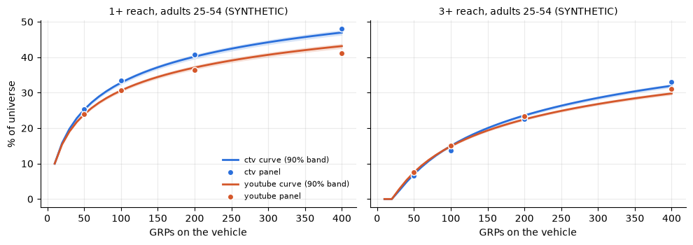
6. Combining vehicles: Sainsbury vs empirical duplication vs truth
Section titled “6. Combining vehicles: Sainsbury vs empirical duplication vs truth”400 GRPs is 200 on each vehicle. Three ways to combine the two 1+ reaches R₁ and R₂:
- Sainsbury (independence): 1 − (1 − R₁)(1 − R₂).
- Empirical duplication: R₁ + R₂ − D·R₁·R₂, where D = P(both) / (P(ctv)·P(youtube)) is read off the clean-room totals. D = 1 is Sainsbury; D > 1 means the audiences overlap more than chance.
- Truth, from the simulation.
For 3+, Sainsbury convolves the two fitted frequency distributions as if independent; the empirical version scales that by the ratio the clean room shows between observed 3+ and the independent prediction among CRM customers. Assumption: the duplication seen among CRM customers carries over to the universe. CRM leans outdoorsy, so this is a declared assumption, not a measurement.
def ratio_3plus(t):    """Observed CRM 3+ over the 3+ that independence predicts from the CRM's own per-vehicle frequencies."""    pa = np.array([t["rows"] - t["seen_a"], t["a_f1"], t["a_f2"]]) / t["rows"]    pb = np.array([t["rows"] - t["seen_b"], t["b_f1"], t["b_f2"]]) / t["rows"]    below = sum(pa[i] * pb[j] for i in range(3) for j in range(3 - i))    return (t["seen_3plus"] / t["rows"]) / (1 - below)

def parts(alpha_beta, t, grps_each=200):    """The pieces every combination is built from: per-vehicle 1+ reach, D, independent 3+ and the 3+ ratio."""    (ac, bc), (ay, by) = alpha_beta    n = spots(grps_each)    below = sum(betabinom.pmf(i, n, ac, bc) * betabinom.pmf(j, n, ay, by) for i in range(3) for j in range(3 - i))    return {"r_ctv": bb_reach(ac, bc, grps_each), "r_yt": bb_reach(ay, by, grps_each), "D": dup_factor(t),            "r3_ind": 1 - below, "ratio3": ratio_3plus(t)}

def dedup(r1, r2, d):    return r1 + r2 - d * r1 * r2

def combine(q):    return {"1+ sainsbury": 1 - (1 - q["r_ctv"]) * (1 - q["r_yt"]), "1+ empirical": dedup(q["r_ctv"], q["r_yt"], q["D"]),            "3+ sainsbury": q["r3_ind"], "3+ empirical": q["r3_ind"] * q["ratio3"]}

point = combine(parts([fits[v]["alpha_beta"] for v in VEHICLES], totals))
# Bootstrap: refit draws for each vehicle, plus clean-room totals redrawn around the released shares# (both / ctv only / youtube only / neither as one multinomial, other counts binomial) with fresh Laplace noise.boot_rng = np.random.default_rng(SEED + 4)n_crm = int(crm_n)sh = {m: min(max(totals[m] / crm_n, 0.0), 1.0) for m in TOTAL_METRICS}draws = []for i in range(BOOT):    both, a_only, b_only, _ = boot_rng.multinomial(n_crm, [sh["seen_both"], sh["seen_a"] - sh["seen_both"],                                                          sh["seen_b"] - sh["seen_both"],                                                          1 - sh["seen_a"] - sh["seen_b"] + sh["seen_both"]])    t = {m: boot_rng.binomial(n_crm, sh[m]) for m in TOTAL_METRICS if m != "rows"}    t.update(seen_both=both, seen_a=both + a_only, seen_b=both + b_only)    t = {m: c + boot_rng.laplace(0, 1 / EPSILON) for m, c in t.items()}    t["rows"] = crm_n    draws.append(parts([fits[v]["boot"][i] for v in VEHICLES], t))part_draws = pd.DataFrame(draws)draws = pd.DataFrame(combine(part_draws))
target = {"1+ sainsbury": truth["combined_reach1_true"], "1+ empirical": truth["combined_reach1_true"], "3+ sainsbury": truth["reach3_combined_true"], "3+ empirical": truth["reach3_combined_true"]}combined = pd.DataFrame({"estimate %": 100 * pd.Series(point), "lo %": 100 * draws.quantile(0.05), "hi %": 100 * draws.quantile(0.95), "truth %": 100 * pd.Series(target)})combined["error pts"] = combined["estimate %"] - combined["truth %"]print(f"duplication factor D from the clean room: {dup_factor(totals):.2f} (1.00 would be independence)")combined.round(1)duplication factor D from the clean room: 1.61 (1.00 would be independence)
| estimate % | lo % | hi % | truth % | error pts | |
|---|---|---|---|---|---|
| 1+ sainsbury | 62.4 | 61.8 | 62.8 | 52.0 | 10.4 |
| 1+ empirical | 53.3 | 52.9 | 53.6 | 52.0 | 1.3 |
| 3+ sainsbury | 42.2 | 41.7 | 42.7 | 37.0 | 5.2 |
| 3+ empirical | 37.5 | 37.0 | 38.1 | 37.0 | 0.6 |
Sainsbury lands near TRUE’s 62% and ten points above the 52% that actually happens. Empirical duplication pulls 1+ back to within about a point and a half, and 3+ to within a point.
Then the setback: neither empirical band reaches the truth. Each carries log sampling and DP noise, nothing else. Two assumptions sit outside it, and UMP asks that an assumption widen the interval it touches (G-EST-02):
- Transfer. D was measured on CRM customers, who lean outdoorsy, and is applied to the whole universe. The room cannot measure the universe’s D, so Sam declares an allowance of ±10% on D and on the 3+ ratio (proposed).
- Curve shape. Section 5 showed the curves miss the panel by up to two points. Each vehicle’s reach is widened by the largest gap the panel showed for it, at any level.
Why an envelope: there are no joint draws of these assumptions, so each bootstrap draw is pushed to the corner that makes reach smallest (and largest), and the 5% and 95% points of those corners are the band.
TRANSFER = 0.10 # proposed allowance on D and the 3+ ratio for the CRM-to-universe transfergap = (coverage["curve %"] - coverage["panel %"]).abs().groupby([coverage.vehicle, coverage.reach]).max() / 100m1c, m1y = gap["ctv", "1+"], gap["youtube", "1+"]m3 = gap["ctv", "3+"] + gap["youtube", "3+"] # both vehicles' 3+ gaps, added: conservativeq = part_drawswidened = { "1+ empirical": (np.quantile(dedup(q.r_ctv - m1c, q.r_yt - m1y, q.D * (1 + TRANSFER)), 0.05), np.quantile(dedup(q.r_ctv + m1c, q.r_yt + m1y, q.D * (1 - TRANSFER)), 0.95)), "3+ empirical": (np.quantile((q.r3_ind - m3) * q.ratio3 * (1 - TRANSFER), 0.05), np.quantile((q.r3_ind + m3) * q.ratio3 * (1 + TRANSFER), 0.95)),}d_universe = (truth["reach1_ctv_200grp"] + truth["reach1_yt_200grp"] - truth["combined_reach1_true"]) / ( truth["reach1_ctv_200grp"] * truth["reach1_yt_200grp"])env = pd.DataFrame({"estimate %": 100 * pd.Series(point)[list(widened)], "sampling lo %": combined.loc[list(widened), "lo %"], "sampling hi %": combined.loc[list(widened), "hi %"], "widened lo %": {k: 100 * v[0] for k, v in widened.items()}, "widened hi %": {k: 100 * v[1] for k, v in widened.items()}, "truth %": combined.loc[list(widened), "truth %"]})env["covers truth"] = env["truth %"].between(env["widened lo %"], env["widened hi %"])print(f"curve allowance (pts): ctv 1+ {100 * m1c:.1f}, youtube 1+ {100 * m1y:.1f}, 3+ combined {100 * m3:.1f}")print(f"D in the CRM {dup_factor(totals):.2f}; D the universe actually had {d_universe:.2f} " f"({100 * (d_universe / dup_factor(totals) - 1):+.0f}%, inside the ±{TRANSFER:.0%} allowance)")env.round(1)curve allowance (pts): ctv 1+ 1.0, youtube 1+ 2.0, 3+ combined 2.5 D in the CRM 1.61; D the universe actually had 1.69 (+5%, inside the ±10% allowance)
| estimate % | sampling lo % | sampling hi % | widened lo % | widened hi % | truth % | covers truth | |
|---|---|---|---|---|---|---|---|
| 1+ empirical | 53.3 | 52.9 | 53.6 | 49.6 | 57.3 | 52.0 | True |
| 3+ empirical | 37.5 | 37.0 | 38.1 | 31.3 | 44.4 | 37.0 | True |
The payoff is a wider, honest band. Both now cover the truth, and the point still sits within the ±3 point target (1+ off by about 1.3 points). Sainsbury stays ten points high whatever band it wears. The universe’s real D landed about 5% above the CRM’s, inside the declared allowance; the room alone could not have told Sam that.
7. Shown numbers with estimands; fin.total only on additive counts
Section titled “7. Shown numbers with estimands; fin.total only on additive counts”Every number Sam hands over gets an estimand. The registry has no reach estimand, so these re-wrap a stand-in:
E-GEO-LIFT-ABS (an absolute lift), with the unit changed to the reach KPI and the family relabelled reach.
Why a re-wrap: fin.estimand takes no metric_family keyword and a kpi override keeps sales_return, so the
dict is edited and wrapped again. Reach is descriptive, not causal: the intervention reads “adding spend (+400)”
where it means 400 GRPs added to the schedule, and the baseline is zero spend (nobody reached). The intervention
types allow only remove_all, scale, add or marginal, so “schedule” cannot be written there.
The CRM counts reuse the same stand-in with a current_plan baseline; their intervention field means nothing,
because whether a customer matches does not depend on the buy.
base = fin.estimand("E-GEO-LIFT-ABS", kpi="reach_1plus", per="absolute", baseline="zero_spend", channels=VEHICLES, weeks=4, intervention="add", size=400, size_kind="absolute", population="exposed")d = base.to_dict()d["metric_family"] = "reach" # no registered reach family; label it plainlyreach_e = fin.estimand(d) # people reached 1+ timesreach3_e = fin.estimand(d, kpi="reach_3plus") # people reached 3+ timespct1_e = fin.estimand(d, kpi="reach_1plus_pct_of_a25_54_universe", per="absolute")pct3_e = fin.estimand(d, kpi="reach_3plus_pct_of_a25_54_universe", per="absolute")crm_e = fin.estimand(d, kpi="crm_customers_matched", baseline="current_plan")overlap_e = fin.estimand(d, kpi="crm_overlap_pct_of_crm_customers", per="absolute", baseline="current_plan")print(reach_e.words)reach 1plus in total from adding spend (+400), exposed, versus zero spend, over 4 weeks, estimator point, 90% confidence
def pct(col, e, label):    """Empirical rows carry the widened band (transfer + curve allowance); Sainsbury keeps its sampling band."""    lo, hi = (100 * w for w in widened[col]) if col in widened else (combined.loc[col, "lo %"], combined.loc[col, "hi %"])    return fin.number(combined.loc[col, "estimate %"], (lo, hi), e, label=label)

shown = { "dedup reach 1+ (people)": fin.number(point["1+ empirical"] * N, tuple(w * N for w in widened["1+ empirical"]), reach_e, label="Deduplicated 1+ reach, 400 GRPs (widened)"), "1+ reach % (empirical)": pct("1+ empirical", pct1_e, "1+ reach, empirical duplication (widened)"), "1+ reach % (Sainsbury)": pct("1+ sainsbury", pct1_e, "1+ reach, Sainsbury (independence; not handed over)"), "3+ reach % (empirical)": pct("3+ empirical", pct3_e, "3+ reach, empirical duplication (widened)"), "3+ reach % (Sainsbury)": pct("3+ sainsbury", pct3_e, "3+ reach, Sainsbury (independence; not handed over)"), "CRM matched, either (people)": fin.number(totals["matched_either"], (totals["matched_either"] - dp_half, totals["matched_either"] + dp_half), crm_e, label="CRM customers reachable at either publisher"), "CRM overlap %": fin.number(100 * overlap, (100 * (totals["matched_both"] - dp_half) / crm_n, 100 * (totals["matched_both"] + dp_half) / crm_n), overlap_e, label="CRM customers at both publishers"),}table(shown)| value | lo | hi | estimand | |
|---|---|---|---|---|
| number | ||||
| dedup reach 1+ (people) | 1066349.3 | 992259.7 | 1146641.8 | reach 1plus in total from adding spend (+400), exposed, versus zero spend, over 4 weeks, estimator point, 90% confidence |
| 1+ reach % (empirical) | 53.3 | 49.6 | 57.3 | reach 1plus pct of a25 54 universe in total from adding spend (+400), exposed, versus zero spend, over 4 weeks, estimator point, 90% confidence |
| 1+ reach % (Sainsbury) | 62.4 | 61.8 | 62.8 | reach 1plus pct of a25 54 universe in total from adding spend (+400), exposed, versus zero spend, over 4 weeks, estimator point, 90% confidence |
| 3+ reach % (empirical) | 37.5 | 31.3 | 44.4 | reach 3plus pct of a25 54 universe in total from adding spend (+400), exposed, versus zero spend, over 4 weeks, estimator point, 90% confidence |
| 3+ reach % (Sainsbury) | 42.2 | 41.7 | 42.7 | reach 3plus pct of a25 54 universe in total from adding spend (+400), exposed, versus zero spend, over 4 weeks, estimator point, 90% confidence |
| CRM matched, either (people) | 112370.0 | 112367.7 | 112372.3 | crm customers matched in total from adding spend (+400), exposed, versus the current plan, over 4 weeks, estimator point, 90% confidence |
| CRM overlap % | 27.3 | 27.3 | 27.3 | crm overlap pct of crm customers in total from adding spend (+400), exposed, versus the current plan, over 4 weeks, estimator point, 90% confidence |
The CRM intervals cover the DP noise only: the CRM is a census, so there is no sampling error, and suppression was corrected by the grand total rather than left in.
Adding counts
Section titled “Adding counts”fin.total adds numbers and builds the dependence envelope. It does not check that the numbers can be added.
Why it matters: the CTV and YouTube reach counts share 25-odd points of the universe. Summed, they describe a plan that reaches more people than exist in its audience. The CRM cells below are disjoint by construction (ctv only, youtube only, both), so they add.
ctv_people = fin.number(bb_reach(*fits["ctv"]["alpha_beta"], 200) * N,                        tuple(np.quantile(bb_reach(fits["ctv"]["boot"][:, 0], fits["ctv"]["boot"][:, 1], 200) * N,                                          [0.05, 0.95])), reach_e, label="CTV 1+ people")yt_people = fin.number(bb_reach(*fits["youtube"]["alpha_beta"], 200) * N,                       tuple(np.quantile(bb_reach(fits["youtube"]["boot"][:, 0], fits["youtube"]["boot"][:, 1], 200)                                         * N, [0.05, 0.95])), reach_e, label="YouTube 1+ people")wrong = fin.total({"ctv": ctv_people, "youtube": yt_people})print(f"WRONG, summed reach: {wrong.value:,.0f} people; deduplicated: {shown['dedup reach 1+ (people)'].value:,.0f}")

def crm_count(n, label):    return fin.number(n, (n - dp_half, n + dp_half), crm_e, label=label)

cells_disjoint = {"ctv only": crm_count(totals["matched_a"] - totals["matched_both"], "CTV only"), "youtube only": crm_count(totals["matched_b"] - totals["matched_both"], "YouTube only"), "both": crm_count(totals["matched_both"], "both")}crm_total = fin.total(cells_disjoint)print(f"disjoint CRM cells add to {crm_total.value:,.0f} ({crm_total.lo:,.0f} to {crm_total.hi:,.0f}, " f"{crm_total.method}); the either-publisher total is {totals['matched_either']:,.0f}")crm_total.to_frame()WRONG, summed reach: 1,544,934 people; deduplicated: 1,066,349 disjoint CRM cells add to 112,372 (112,365 to 112,379, per_channel_envelope); the either-publisher total is 112,370
| lo | hi | |
|---|---|---|
| independent | 112368.011806 | 112375.988194 |
| comonotone | 112365.092245 | 112378.907755 |
| reported | 112365.092245 | 112378.907755 |
8. A reach_frequency Tier D manifest with the duplication assumption declared
Section titled “8. A reach_frequency Tier D manifest with the duplication assumption declared”The Tier D summary shape only knows roi and mroi, so the per-vehicle reach counts sit under the roi label
while reach_e carries their meaning. The curves live in an extra doc key (reach_curves); the declared duplication,
suppression floor and ε go in notes; the hand-run panel coverage goes in the identification layer of acceptance.
curves_doc = {v: {"model": "beta_binomial_mom", "grp_per_spot": GRP_PER_SPOT, "alpha": float(fits[v]["alpha_beta"][0]), "beta": float(fits[v]["alpha_beta"][1]), "grps": LEVELS, "reach_1plus": [float(bb_reach(*fits[v]["alpha_beta"], g)) for g in LEVELS], "reach_3plus": [float(bb_reach(*fits[v]["alpha_beta"], g, 3)) for g in LEVELS]} for v in VEHICLES}n_cov, n_lv = int(coverage.covered.sum()), len(coverage)m = fin.Model.from_table( {"ctv": ctv_people, "youtube": yt_people}, estimand=reach_e, name="nw_rf_ctv_yt", engine="beta-binomial", client="northwind-outdoor", family="reach_frequency", metric="roi", dependence="declared_assumption", notes=[{"duplication": "empirical clean-room overlap", "duplication_factor": round(float(dup_factor(totals)), 3), "transfer_allowance_on_D": TRANSFER, "curve_allowance": "largest panel gap per vehicle", "suppression_k": K, "dp_epsilon": EPSILON, "thresholds": "proposed, illustrative", "summary_label": "roi slot holds 1+ reach people at 200 GRPs per vehicle; see estimand"}], reach_curves=curves_doc, acceptance={"status": "untested", "identification": { "status": "passed" if n_cov == n_lv else "untested", "metrics": {"panel_coverage": f"{n_cov} of {n_lv} vehicle x level x 1+/3+ points", "run": "by hand in notebook 12; no gate checks it"}}},)check = m.check()check.to_frame()[["gate", "outcome", "message"]]| gate | outcome | message | |
|---|---|---|---|
| 0 | G-ACC-01 | fallback | acceptance untested: usable, labelled unvalidated method, trust reduced |
| 1 | G-CAP-01 | route | sandbox output: experimental label and a named approver needed |
G-ACC-01 labels the method unvalidated (no acceptance report backs it) and G-CAP-01 routes the sandbox output to a
named approver. Neither blocks. Nothing family-specific runs: UMP does not yet enforce the §16 reach and frequency
check, which is why it sits in acceptance as a hand-run record.
Two last privacy checks before release, on the manifest itself:
cells = {"segments": [{"id": "R01|25-34", "size": 4100}],         "aggregate": {"query": "reach by region x age band", "n": 4100}}small = {**cells, "destination": "client", "segments": [*cells["segments"], {"id": "R58|45-54", "size": 31}]}try:    fin.check("model_manifest", m.doc, operation="release", context=small).raise_for_stops()except fin.Stopped as stop:    print(stop.code, "|", stop)
leaky = {**m.doc, "notes": [*m.doc.get("notes", []), {"hashed_ids": ["9f2c...", "a71b..."]}]} # undeclared members are refused (§21)export = {**cells, "citations": []} # an export states what it cites; this offline manifest cites nonetry: fin.check("model_manifest", leaky, operation="export", context={**export, "destination": "client"}).raise_for_stops()except fin.Stopped as stop: print(stop.code, "|", stop)inside = fin.check("model_manifest", leaky, operation="export", context={**export, "destination": "clean_room"})print("destination clean_room:", inside)PRIVACY_FLOOR | PRIVACY_FLOOR: G-PRIV-01: 1 segment(s) below minimum size 50 PRIVACY_FLOOR | PRIVACY_FLOOR: G-PRIV-02: member-level fields ['hashed_ids'] would leave to client destination clean_room: <GateReport Would pass · 0 stops · 1 fallbacks · 0 warnings · 15 gates (2 fired)>
9. Going deeper
Section titled “9. Going deeper”- Better curves. A beta-binomial with a zero-inflation term (people with no account) would likely fix the far-out misses; so would fitting on two past flights instead of one.
- Duplication by segment. The clean room can return D by age band; applying it per band and summing (disjoint bands add) weakens the CRM-represents-universe assumption.
- Noise budget. ε here is per count; the total spent composes across counts. A real room tracks that; this stand-in only tracks the number of releases.
- The profile check. Panel coverage is a §16 acceptance check that no gate runs yet. Notebook 02 shows how gates are wired; a reach and frequency profile would add one.
What Sam handed over
Section titled “What Sam handed over”| Asked | CRM reach at two publishers; what 400 GRPs (200 CTV + 200 YouTube) buys among adults 25-54 |
| Handed over | see the two lines printed below, each with its estimand and 90% interval |
| Assumed | CRM duplication carries to the universe within ±10% (declared, declared_assumption, proposed); reach is descriptive, on a stand-in estimand; k = 50 and ε = 1 are proposed |
| Fell back | suppressed cells corrected by the noised grand total (disclosed); acceptance untested (G-ACC-01), sandbox route (G-CAP-01); reach bands widened on an envelope for the transfer allowance and the panel’s curve gaps (G-EST-02, G-DEP-01) |
| Next | refit the curve with a no-account term before quoting anything above 200 GRPs a vehicle; ask the room for D by age band |
for key in ["dedup reach 1+ (people)", "1+ reach % (empirical)", "3+ reach % (empirical)", "CRM matched, either (people)", "CRM overlap %"]: a = shown[key] print(f"{a.label}: {a.value:,.1f} (90% {a.lo:,.1f} to {a.hi:,.1f}); {a.estimand.words}")Deduplicated 1+ reach, 400 GRPs (widened): 1,066,349.3 (90% 992,259.7 to 1,146,641.8); reach 1plus in total from adding spend (+400), exposed, versus zero spend, over 4 weeks, estimator point, 90% confidence 1+ reach, empirical duplication (widened): 53.3 (90% 49.6 to 57.3); reach 1plus pct of a25 54 universe in total from adding spend (+400), exposed, versus zero spend, over 4 weeks, estimator point, 90% confidence 3+ reach, empirical duplication (widened): 37.5 (90% 31.3 to 44.4); reach 3plus pct of a25 54 universe in total from adding spend (+400), exposed, versus zero spend, over 4 weeks, estimator point, 90% confidence CRM customers reachable at either publisher: 112,370.0 (90% 112,367.7 to 112,372.3); crm customers matched in total from adding spend (+400), exposed, versus the current plan, over 4 weeks, estimator point, 90% confidence CRM customers at both publishers: 27.3 (90% 27.3 to 27.3); crm overlap pct of crm customers in total from adding spend (+400), exposed, versus the current plan, over 4 weeks, estimator point, 90% confidence
Next: notebook 02 (02 · Validate and gate a document offline) for how the gates you met here are evaluated, and notebook 04 (04 · ump-core from a notebook) to file this manifest with ump-core.