06 · scikit-learn pipelines and business questions
You will learn
- Build adstock, saturation and seasonality transformers for a Pipeline
- Bootstrap the whole workflow, tuning included
- Answer named business questions, each with its own estimand
- Run the workflow twice and get the same answers
You need
- Python 3.12 and uv
- Some scikit-learn (Pipeline, GridSearchCV)
Runs offline. Uses babelfin, finprint and scikit-learn. The data is SYNTHETIC, generated in the first
cells with a known truth, so we can check every answer against it.
Northwind’s analytics team has a standard toolkit: pandas for prep, scikit-learn for models. Every quarter they rebuild the same model and answer the same handful of questions for the media lead. Every quarter something drifts: a cleaning step done by hand, a hyperparameter someone tweaked, a “ROI” that was really a marginal ROI.
This notebook keeps their toolkit and makes the workflow repeatable end to end:
- prep recorded with
finprint, so the model’s input has a replayable recipe; - an sklearn
Pipelinewith custom transformers (adstock, saturation, seasonality), hyperparameters chosen by time-series cross-validation; - uncertainty from a moving-block bootstrap of the fitted pipeline;
- named business questions: small registered functions that turn the fitted model into answers, each with its own estimand, so “what did TV return?” and “what does the next TV dollar return?” can never be confused;
- the whole workflow as one function, run twice to show it gives the same answers.
%load_ext finprintfrom collections.abc import Callablefrom dataclasses import dataclassfrom pathlib import Path
import babelfin as finimport finprint as fpimport matplotlib.pyplot as pltimport numpy as npimport pandas as pdfrom sklearn.base import BaseEstimator, TransformerMixinfrom sklearn.compose import ColumnTransformerfrom sklearn.linear_model import LinearRegressionfrom sklearn.model_selection import GridSearchCV, ParameterGrid, TimeSeriesSplitfrom sklearn.pipeline import Pipeline
OUT = Path("out")OUT.mkdir(exist_ok=True)CHANNELS = ["tv", "search", "social"]SEED = 11
0. A synthetic world with a known truth
Section titled “0. A synthetic world with a known truth”Three years of weekly sales with carryover (adstock) and diminishing returns (saturation). The raw file has the usual problems: a duplicated week from the feed and one missing search week. The truth is kept aside for checking.
TRUE = {"decay": {"tv": 0.5, "search": 0.0, "social": 0.3}, "slope": {"tv": 1.8, "search": 3.0, "social": 2.4},        "half_sat_mult": 1.0}   # each channel's half-saturation point is this times its mean adstocked spend

def adstock(x, decay):    out = np.zeros(len(x))    for t, v in enumerate(x):        out[t] = v + (decay * out[t - 1] if t else 0.0)    return out

def saturate(a, k):    return k * np.log1p(a / k)            # slope 1 at zero spend, flattening as spend grows

def make_world(seed=SEED, weeks=156):    rng = np.random.default_rng(seed)    week = pd.date_range("2023-01-02", periods=weeks, freq="W-MON")    spend = pd.DataFrame({"tv": rng.gamma(4, 9000, weeks), "search": rng.gamma(5, 2500, weeks),                          "social": rng.gamma(3, 4000, weeks)}).round(2)    promo = (np.arange(weeks) % 9 == 3).astype(int)    t = np.arange(weeks)    ads = {c: adstock(spend[c].to_numpy(), TRUE["decay"][c]) for c in CHANNELS}    contrib = {c: TRUE["slope"][c] * saturate(ads[c], TRUE["half_sat_mult"] * ads[c].mean()) for c in CHANNELS}    sales = 200_000 + 30_000 * np.sin(2 * np.pi * t / 52) + 15_000 * promo + sum(contrib.values())    sales = sales + rng.normal(0, 8_000, weeks)    raw = pd.DataFrame({"week": week.strftime("%Y-%m-%d"), "sales": sales.round(2), **spend, "promo": promo})    raw.loc[40, "search"] = np.nan                       # a missing week in the feed    raw = pd.concat([raw.iloc[:20], raw.iloc[[19]], raw.iloc[20:]], ignore_index=True)   # a duplicated week    truth_roi = {c: contrib[c].sum() / spend[c].sum() for c in CHANNELS}    return raw, truth_roi

raw_frame, TRUTH_ROI = make_world()raw_frame.to_csv(OUT / "sk_raw.csv", index=False)raw_frame.head()| week | sales | tv | search | social | promo | |
|---|---|---|---|---|---|---|
| 0 | 2023-01-02 | 289765.35 | 33592.78 | 4362.40 | 11666.25 | 0 |
| 1 | 2023-01-09 | 357400.09 | 58926.07 | 14329.35 | 9511.26 | 0 |
| 2 | 2023-01-16 | 379233.63 | 28126.64 | 22913.72 | 25251.23 | 0 |
| 3 | 2023-01-23 | 370137.68 | 43824.44 | 12634.67 | 9889.48 | 1 |
| 4 | 2023-01-30 | 375249.09 | 47617.64 | 8001.33 | 20643.60 | 0 |
1. Prep, recorded
Section titled “1. Prep, recorded”Ordinary pandas through a finprint session: the recipe beside the clean file says exactly what was done, and
verify replays it.
rec = fin.record("northwind sklearn prep (synthetic data)")raw = rec.read_csv(OUT / "sk_raw.csv", parse_dates=["week"])clean = raw.drop_duplicates(subset=["week"])clean = clean.sort_values("week")clean["search"] = clean["search"].interpolate()clean = clean.reset_index(drop=True)saved = rec.save(clean, OUT / "sk_model_input.csv")print(fin.verify_recipe(saved.recipe_path, inputs_dir=OUT).message)print("\n".join(fp.describe(saved.recipe)))Reproduced: 4 steps from 1 inputs. Dropped 1 row that were duplicates: 157 to 156 [cell 3] Sorted by 'week' [cell 3] Filled gaps in search by interpolation [cell 3] Moved the index into columns [cell 3]
2. The model as an sklearn Pipeline
Section titled “2. The model as an sklearn Pipeline”Media effects get their own transformer, so carryover and saturation are part of the model, not a hand-made
column somebody forgets to rebuild. Hyperparameters (the decay per channel and how fast returns flatten) are
ordinary pipeline parameters, so GridSearchCV with TimeSeriesSplit picks them on data the fit has not seen.
class MediaTransform(BaseEstimator, TransformerMixin):    """Adstock then saturation, per channel. ``k_mult`` scales each channel's half-saturation point from its mean    adstocked spend (learned in ``fit``). Carryover needs the weeks before: ``fit`` keeps the spend it saw, and    ``transform`` prepends the earlier weeks it knows, so a later week (a CV test fold, next quarter's data) starts    with the carryover it really had. Only past spend is used, never sales, so nothing leaks."""
    def __init__(self, tv_decay=0.5, search_decay=0.0, social_decay=0.3, k_mult=1.0):        self.tv_decay, self.search_decay, self.social_decay, self.k_mult = tv_decay, search_decay, social_decay, k_mult
    def _adstocked(self, X):        known = getattr(self, "history_", None)        earlier = known[known["week"] < X["week"].min()] if known is not None else X.iloc[:0]        full = pd.concat([earlier, X[["week", *CHANNELS]]], ignore_index=True)        n = len(earlier)        return {c: adstock(full[c].to_numpy(dtype=float), getattr(self, f"{c}_decay"))[n:] for c in CHANNELS}
    def fit(self, X, y=None):        self.history_ = None        self.k_ = {c: self.k_mult * a.mean() for c, a in self._adstocked(X).items()}        self.history_ = X[["week", *CHANNELS]].copy()        return self
    def transform(self, X):        return np.column_stack([saturate(a, self.k_[c]) for c, a in self._adstocked(X).items()])
    def get_feature_names_out(self, input_features=None):        return np.array(CHANNELS, dtype=object)

class Seasonality(BaseEstimator, TransformerMixin):    """A yearly cycle and a trend from the week column."""
    def fit(self, X, y=None):        self.start_ = pd.to_datetime(X["week"]).min()        return self
    def transform(self, X):        t = (pd.to_datetime(X["week"]) - self.start_).dt.days.to_numpy() / 7.0        return np.column_stack([np.sin(2 * np.pi * t / 52), np.cos(2 * np.pi * t / 52), t / 52])
    def get_feature_names_out(self, input_features=None):        return np.array(["season_sin", "season_cos", "trend"], dtype=object)

def make_pipeline():    features = ColumnTransformer([("media", MediaTransform(), ["week", *CHANNELS]),                                  ("season", Seasonality(), ["week"]),                                  ("promo", "passthrough", ["promo"])])    return Pipeline([("features", features), ("model", LinearRegression())])

GRID = {"features__media__tv_decay": [0.3, 0.5, 0.7], "features__media__social_decay": [0.0, 0.3, 0.5],        "features__media__search_decay": [0.0, 0.3], "features__media__k_mult": [0.5, 1.0, 2.0]}
data = fp.untrack(clean)X, y = data[["week", *CHANNELS, "promo"]], data["sales"]search = GridSearchCV(make_pipeline(), GRID, cv=TimeSeriesSplit(n_splits=5), scoring="neg_mean_absolute_percentage_error")search.fit(X, y)print("chosen:", {k.split("__")[-1]: v for k, v in search.best_params_.items()})print(f"cross-validated MAPE {-search.best_score_:.1%} (folds: " + ", ".join(f"{-s:.1%}" for s in [search.cv_results_[f"split{i}_test_score"][search.best_index_] for i in range(5)]) + ")")chosen: {'k_mult': 2.0, 'search_decay': 0.3, 'social_decay': 0.3, 'tv_decay': 0.5}
cross-validated MAPE 2.6% (folds: 4.3%, 2.0%, 3.3%, 1.1%, 2.2%)
Why MediaTransform keeps the spend it saw: a CV test fold starts in the middle of the series. Restarting the
adstock at zero there would penalise long carryover and bias the search toward short decays. Prepending the
earlier weeks’ spend gives each fold the carryover it really had, using spend only (known in advance), never sales.
3. Uncertainty: bootstrap the whole workflow, tuning included
Section titled “3. Uncertainty: bootstrap the whole workflow, tuning included”Decay, saturation and slope trade off against each other, and “remove all spend” extrapolates to zero spend, where that trade-off matters most. Holding the tuned values fixed would hide it. So each bootstrap draw:
- resamples 8-week blocks of the series (weeks stay in order inside a block);
- picks its own decays and saturation by error on the weeks it left out (out-of-bag);
- refits the regression on its resample.
Features for every grid point are built once on the full series (carryover needs the weeks in order), so 300
draws over 54 grid points still run in seconds. Everything a question needs goes into one FittedModel, so
answering never reaches for a global.
@dataclassclass FittedModel:    X: pd.DataFrame    features: list          # one fitted features step per grid point    draws: list             # (grid point index, fitted regression) per bootstrap draw
    @property    def weeks(self):        return len(self.X)
    @property    def spend(self):        return {c: float(self.X[c].sum()) for c in CHANNELS}
    def sales(self, **spend):        """Weekly sales for every draw (draws x weeks) with some channels' weekly spend replaced. Each draw's own        features step rebuilds adstock and saturation from the new spend, so carryover follows the change."""        Xs = self.X.assign(**spend)        F = {i: self.features[i].transform(Xs) for i in {i for i, _ in self.draws}}        return np.stack([m.predict(F[i]) for i, m in self.draws])
    @property    def base(self):        return self.sales()
    def chosen(self):        """How often each grid point was chosen across draws: the tuning uncertainty, made visible."""        counts = pd.Series([i for i, _ in self.draws]).value_counts()        return pd.DataFrame([{**{k.split("__")[-1]: v for k, v in GRID_POINTS[i].items()}, "share": n / len(self.draws)}                             for i, n in counts.items()])

GRID_POINTS = list(ParameterGrid(GRID))

def fit_model(X, y, seed=SEED, n_draws=300, block=8):    features = [make_pipeline().set_params(**p).named_steps["features"].fit(X) for p in GRID_POINTS]    F = [f.transform(X) for f in features]    yv, n = y.to_numpy(), len(y)    rng = np.random.default_rng(seed)    starts = np.arange(n - block + 1)    draws = []    for _ in range(n_draws):        rows = np.concatenate([np.arange(s, s + block) for s in rng.choice(starts, n // block + 1)])[:n]        oob = np.setdiff1d(np.arange(n), rows)        fits = [LinearRegression().fit(Fi[rows], yv[rows]) for Fi in F]        errs = [np.mean(np.abs(m.predict(Fi[oob]) - yv[oob]) / yv[oob]) for m, Fi in zip(fits, F)]        best = int(np.argmin(errs))        draws.append((best, fits[best]))    return FittedModel(X, features, draws)

fitted = fit_model(X, y)fitted.chosen().sort_values("share", ascending=False).head(6).round(2)| k_mult | search_decay | social_decay | tv_decay | share | |
|---|---|---|---|---|---|
| 0 | 0.5 | 0.0 | 0.3 | 0.5 | 0.39 |
| 1 | 1.0 | 0.0 | 0.3 | 0.5 | 0.26 |
| 2 | 2.0 | 0.0 | 0.3 | 0.5 | 0.12 |
| 3 | 0.5 | 0.0 | 0.3 | 0.3 | 0.09 |
| 4 | 0.5 | 0.3 | 0.3 | 0.3 | 0.05 |
| 5 | 1.0 | 0.0 | 0.3 | 0.3 | 0.01 |
The draws spread over several grid points, and cross-validation’s single winner above is only one of them. The data can tell the decays apart better than the saturation, so the saturation stays uncertain, and the answers’ intervals carry that uncertainty instead of hiding it.
4. Named business questions
Section titled “4. Named business questions”Each question is a small registered function: a name, the question in words, the estimand that says exactly what the number means, and the code that answers it from a fitted model. The registry is the team’s shared vocabulary: next quarter the same names give the same kind of answer, and nobody reports a marginal return as an average one.
@dataclassclass Question:    name: str    ask: str    estimand: fin.Estimand    answer: Callable[[FittedModel], np.ndarray]      # one value per bootstrap draw

QUESTIONS: dict[str, Question] = {}

def question(name, ask, estimand):    def register(fn):        QUESTIONS[name] = Question(name, ask, estimand, fn)        return fn    return register

COMMON = {"kpi": "incremental_sales", "cost_basis": "gross", "point_rule": "posterior_median",          "interval": "bootstrap_pct", "weeks": 156}
for ch in CHANNELS:    @question(f"roi_{ch}", f"What did each dollar of {ch} return over the three years?",              fin.estimand("roi", channels=ch, **COMMON))    def _roi(m, ch=ch):        return (m.base - m.sales(**{ch: 0.0})).sum(axis=1) / m.spend[ch]
    @question(f"mroi_{ch}", f"What would the next dollar of {ch} return?",              fin.estimand("mroi", channels=ch, **COMMON))    def _mroi(m, ch=ch):        return (m.sales(**{ch: m.X[ch] * 1.1}) - m.base).sum(axis=1) / (0.1 * m.spend[ch])

@question("cut_tv_20pct", "What happens to sales if we cut TV by 20%?",          fin.estimand("roi", channels="tv", intervention="scale", size=-0.2, baseline="current_plan",                       per="absolute", **COMMON))def _cut_tv(m):    return (m.sales(tv=m.X["tv"] * 0.8) - m.base).sum(axis=1)

@question("move_tv_to_search", "What if we move 20% of TV spend to search?",          fin.estimand("roi", intervention={"type": "scale", "size": -0.2, "size_kind": "relative",                                            "arms": ["from:tv", "to:search"]},                       baseline="current_plan", per="absolute", **COMMON))def _move(m):    moved = 0.2 * m.X["tv"]                       # 20% of each week's TV budget goes to search    return (m.sales(tv=m.X["tv"] - moved, search=m.X["search"] + moved) - m.base).sum(axis=1)

pd.DataFrame([{"name": q.name, "asks": q.ask, "means": q.estimand.words} for q in QUESTIONS.values()])| name | asks | means | |
|---|---|---|---|
| 0 | roi_tv | What did each dollar of tv return over the thr... | incremental sales per dollar, gross from remov... |
| 1 | mroi_tv | What would the next dollar of tv return? | incremental sales per dollar, gross from a sma... |
| 2 | roi_search | What did each dollar of search return over the... | incremental sales per dollar, gross from remov... |
| 3 | mroi_search | What would the next dollar of search return? | incremental sales per dollar, gross from a sma... |
| 4 | roi_social | What did each dollar of social return over the... | incremental sales per dollar, gross from remov... |
| 5 | mroi_social | What would the next dollar of social return? | incremental sales per dollar, gross from a sma... |
| 6 | cut_tv_20pct | What happens to sales if we cut TV by 20%? | incremental sales in total, gross from scaling... |
| 7 | move_tv_to_search | What if we move 20% of TV spend to search? | incremental sales in total, gross from moving ... |
Answer them all. Each answer is a fin.Number: the median of the draws with a 90% bootstrap interval (tuning
included), carrying its estimand.
def answer_all(m, level=0.9):    out = {}    for q in QUESTIONS.values():        d = q.answer(m)        lo, hi = np.quantile(d, [(1 - level) / 2, (1 + level) / 2])        out[q.name] = fin.number(float(np.median(d)), (float(lo), float(hi)), q.estimand, label=q.ask)    return out

answers = answer_all(fitted)pd.DataFrame([{"question": n, "value": a.value, "lo": a.lo, "hi": a.hi, "in words": a.words} for n, a in answers.items()]).round(2)| question | value | lo | hi | in words | |
|---|---|---|---|---|---|
| 0 | roi_tv | 2.22 | 1.87 | 2.68 | 2.22, likely between 1.87 and 2.68 |
| 1 | mroi_tv | 1.52 | 1.14 | 1.63 | 1.52, likely between 1.14 and 1.63 |
| 2 | roi_search | 1.72 | 1.37 | 2.32 | 1.72, likely between 1.37 and 2.32 |
| 3 | mroi_search | 1.11 | 0.90 | 1.44 | 1.11, likely between 0.90 and 1.44 |
| 4 | roi_social | 2.62 | 2.08 | 2.99 | 2.62, likely between 2.08 and 2.99 |
| 5 | mroi_social | 1.65 | 1.50 | 1.81 | 1.65, likely between 1.50 and 1.81 |
| 6 | cut_tv_20pct | -1898520.95 | -2038710.16 | -1444957.32 | -1,898,521, likely between -2.0M and -1.4M |
| 7 | move_tv_to_search | -663707.44 | -960426.55 | -48026.87 | -663,707, likely between -960K and -48K |
Did the model get it right?
Section titled “Did the model get it right?”The world is synthetic, so the true average ROI is known. The intervals should cover it.
check = pd.DataFrame([{"channel": c, "estimate": answers[f"roi_{c}"].value, "lo": answers[f"roi_{c}"].lo, "hi": answers[f"roi_{c}"].hi, "truth": TRUTH_ROI[c]} for c in CHANNELS])check["covered"] = (check.lo <= check.truth) & (check.truth <= check.hi)check.round(3)| channel | estimate | lo | hi | truth | covered | |
|---|---|---|---|---|---|---|
| 0 | tv | 2.224 | 1.870 | 2.682 | 2.457 | True |
| 1 | search | 1.721 | 1.372 | 2.324 | 2.014 | True |
| 2 | social | 2.616 | 2.078 | 2.995 | 2.290 | True |
fig, ax = plt.subplots(figsize=(7, 2.6))for i, c in enumerate(CHANNELS): for j, (kind, color) in enumerate([("roi", "#5b8def"), ("mroi", "#e8833a")]): a = answers[f"{kind}_{c}"] ax.plot([a.lo, a.hi], [i + 0.15 * (j - 0.5)] * 2, lw=5, color=color, solid_capstyle="butt", label=("average ROI" if kind == "roi" else "next-dollar mROI") if i == 0 else None) ax.plot(TRUTH_ROI[c], i - 0.075, "kx")ax.set_yticks(range(len(CHANNELS)), CHANNELS)ax.set_xlabel("sales per $1 (90% bootstrap interval); x = true average ROI")ax.legend(fontsize=8, loc="lower right")plt.tight_layout()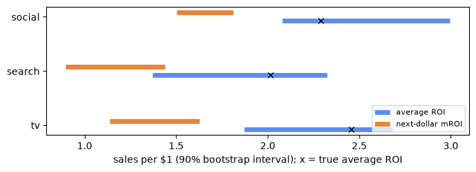
Same channel, two different questions
Section titled “Same channel, two different questions”With diminishing returns the next dollar earns less than the average dollar. Ask babelfin whether the two can be combined: they cannot, because one removes all spend and the other adds a little. They go side by side.
fin.compare(answers["roi_tv"], answers["mroi_tv"])details
| why | a remove-all (ROI) and a marginal (mROI) intervention answer different questions |
|---|
| field | first | second |
|---|---|---|
| intervention | type remove_all, size -1.0, size_kind relative, arms , population geo_set | type marginal, size 0.1, size_kind relative, arms , population geo_set |
| baseline | zero_spend | current_plan |
The two budget scenarios, as the media lead would read them. When an interval spans zero, the honest answer is that the data cannot tell whether the move helps.
answers["cut_tv_20pct"]details
| means | incremental sales in total, gross from scaling spend (-20%), geo_set, versus the current plan, over 156 weeks, posterior median, 90% bootstrap_pct |
|---|---|
| interval | 90% bootstrap_pct -2,038,710 to -1,444,957 |
| trust level | 2 |
answers["move_tv_to_search"]details
| means | incremental sales in total, gross from moving 20% of tv spend from tv to search (total unchanged), versus the current plan, over 156 weeks, posterior median, 90% bootstrap_pct |
|---|---|
| interval | 90% bootstrap_pct -960,427 to -48,027 |
| trust level | 2 |
5. Package the answers as a model
Section titled “5. Package the answers as a model”The average ROIs become a Tier D model with their estimand, joint-draws dependence and a link to the prep recipe, checked against the gates the platform will run. Notebook 04 shows how to file it.
model = fin.Model.from_table( pd.DataFrame([{"channel": c, "value": answers[f"roi_{c}"].value, "lo": answers[f"roi_{c}"].lo, "hi": answers[f"roi_{c}"].hi, "current_spend": fitted.spend[c]} for c in CHANNELS]), estimand=fin.estimand("roi", channels=CHANNELS, **COMMON), name="Northwind sklearn MMM (synthetic data)", engine="sklearn:LinearRegression", dependence="joint_draws", recipe=saved)model.check()details
| gate | outcome | message | codes |
|---|---|---|---|
| G-ACC-01 | fallback | acceptance untested: usable, labelled unvalidated method, trust reduced | UNVALIDATED_METHOD |
| G-CAP-01 | route | sandbox output: experimental label and a named approver needed | EXPERIMENTAL_LABEL |
6. The whole workflow, twice
Section titled “6. The whole workflow, twice”Everything above as one function with no hidden state: the raw file in, the answers out. Seeds are fixed, the prep is recorded, and the tuning happens inside the bootstrap the same way every time. Running it twice from scratch and comparing is the cheapest repeatability test there is.
def run_workflow(raw_csv, seed=SEED):    r = fin.record("workflow run")    df = r.read_csv(raw_csv, parse_dates=["week"]).drop_duplicates(subset=["week"]).sort_values("week")    df["search"] = df["search"].interpolate()    df = fp.untrack(df.reset_index(drop=True))    m = fit_model(df[["week", *CHANNELS, "promo"]], df["sales"], seed=seed)    return pd.DataFrame({n: [a.value, a.lo, a.hi] for n, a in answer_all(m).items()}, index=["value", "lo", "hi"]).T

first, second = run_workflow(OUT / "sk_raw.csv"), run_workflow(OUT / "sk_raw.csv")print("identical answers on a second run from scratch:", first.equals(second))first.round(2)identical answers on a second run from scratch: True
| value | lo | hi | |
|---|---|---|---|
| roi_tv | 2.22 | 1.87 | 2.68 |
| mroi_tv | 1.52 | 1.14 | 1.63 |
| roi_search | 1.72 | 1.37 | 2.32 |
| mroi_search | 1.11 | 0.90 | 1.44 |
| roi_social | 2.62 | 2.08 | 2.99 |
| mroi_social | 1.65 | 1.50 | 1.81 |
| cut_tv_20pct | -1898520.95 | -2038710.16 | -1444957.32 |
| move_tv_to_search | -663707.44 | -960426.55 | -48026.87 |
What you have now
Section titled “What you have now”out/sk_model_input.csvwith its recipe: the prep, replayed and verified.- A scikit-learn pipeline whose carryover, saturation and seasonality are model steps with tuned parameters.
- A registry of named questions, each answer a
fin.Numberwith its estimand and interval. - A Tier D model ready to file (notebook 04), and a workflow function that gives the same answers every run.
Next: save this workflow, rerun it and share it in 07 (07 · A scikit-learn workflow: build it, save it, share it): the same model in a module, saved as a bundle that scores new weeks, and approved once so colleagues and a served app can run it.