10 · Who buys anyway: propensity vs uplift audiences

You will learn

• Tell a response (propensity) model from an uplift model
• Read Qini curves and AUUC on a randomised holdout
• Hand over uplift at the top 20% with its estimand and interval
• File a Tier D audience model and meet the segment-size privacy stop

You need

• Python 3.12 and uv
• Some scikit-learn (classifiers)

Run this notebook Offline

notebooks/10_audience_uplift_vs_propensity.ipynb

Runs offline on your laptop. The outputs on this page were saved from a real run.

About 25 minutes

Access needed. The packages and notebooks are not yet publicly distributed. The steps below need a checkout of the UMP repository. Pages show recorded outputs, so you can follow along without running them.

cd notebooks && uv run jupyter lab

Runs offline. Uses babelfin and scikit-learn. The users are SYNTHETIC, generated below with a known truth.

Northwind Outdoor wants a “high-value hikers” audience for its spring Meta push, and Maya Chen has to prove it beats broad targeting. Her first model looks great: a propensity score with a strong AUC whose top decile converts at several times the base rate. Then Sam Patel asks the only question that pays for media: what did the ads add?

This notebook follows Maya from that false start to an uplift audience she can hand over, with the estimand beside the number, a pilot label on the model, and a privacy stop before anything leaves the building.

In [1]:

import babelfin as fin
import matplotlib.pyplot as plt
import numpy as np
import pandas as pd
from sklearn.ensemble import GradientBoostingClassifier
from sklearn.linear_model import LogisticRegression
from sklearn.metrics import roc_auc_score

SEED = 14                                  # see the note in section 4 on seeds
K = 0.20                                   # share of users Northwind will target
pd.set_option("display.max_colwidth", None)

1. The ask, and a false start

Maya’s brief: rank Northwind’s users, hand Meta the top 20%. The first instinct is a response model, “who is likely to buy”. Section 3 builds it. Before that, the world it runs in.

2. Synthetic users with a known truth

Four latent types, the classic uplift quadrants. Nobody sees the type; the features only hint at it. Ads are randomised: half the users were eligible for the Meta flight, half were held out.

In [2]:

TRUE = {
    "segments": {   # share of users, conversion rate without ads, extra conversion rate from ads
        "loyalists":     {"share": 0.25, "base": 0.150, "uplift": 0.000},
        "persuadables":  {"share": 0.20, "base": 0.030, "uplift": 0.030},
        "lost_causes":   {"share": 0.45, "base": 0.005, "uplift": 0.000},
        "sleeping_dogs": {"share": 0.10, "base": 0.050, "uplift": -0.010},
    },
    "treat_share": 0.5, "n_users": 200_000, "holdout_share": 0.30,
}
seg = TRUE["segments"]
TRUE["base_rate"] = sum(s["share"] * s["base"] for s in seg.values())
TRUE["oracle_at_k"] = 1000 * seg["persuadables"]["uplift"]                  # top 20% = exactly the persuadables
TRUE["random_at_k"] = 1000 * sum(s["share"] * s["uplift"] for s in seg.values())
{k: round(v, 4) for k, v in TRUE.items() if k not in ("segments",)}

Out [2]:

{'treat_share': 0.5,
 'n_users': 200000,
 'holdout_share': 0.3,
 'base_rate': 0.0508,
 'oracle_at_k': 30.0,
 'random_at_k': 5.0}

Per 1,000 users targeted, a perfect ranking adds 30 conversions at k = 20%; a random 20% adds 5.

Why 200,000 users: with 60,000 the holdout’s top 20% is about 3,600 people, and the 90% interval on uplift spans roughly ±11 per 1,000. That is too wide to separate a good ranking from a lucky one, so the synthetic world is larger. A real pilot would size the holdout the same way, before the flight.

In [3]:

def make_users(seed=SEED):
    rng = np.random.default_rng(seed)
    names = list(seg)
    n = TRUE["n_users"]
    typ = rng.choice(len(names), n, p=[seg[k]["share"] for k in names])
    pick = lambda vals: np.array(vals)[typ]  # (one value per type, in TRUE's order)
    users = pd.DataFrame({
        "age": np.clip(pick([44, 33, 40, 47]) + rng.normal(0, 9, n), 18, 80).round(),
        "rural": rng.binomial(1, 0.12, n),
        "climber": rng.binomial(1, pick([0.004, 0.008, 0.002, 0.003])),
        "past_orders": rng.poisson(pick([4.0, 0.3, 0.3, 1.8])),
        "days_since_visit": np.clip(rng.gamma(2, pick([8, 20, 60, 25])), 0, 365).round(),
        "hiking_interest": (pick([0.4, 1.4, -0.4, 0.3]) + rng.normal(0, 0.5, n)).round(2),
        "email_opt_out": rng.binomial(1, pick([0.05, 0.04, 0.08, 0.70])),
        "treat": rng.binomial(1, TRUE["treat_share"], n),
    })
    true_uplift = pick([seg[k]["uplift"] for k in names])
    users["converted"] = rng.binomial(1, pick([seg[k]["base"] for k in names]) + users["treat"] * true_uplift)
    users["holdout"] = rng.random(n) < TRUE["holdout_share"]
    return users, true_uplift, np.array(names)[typ]


users, true_uplift, true_type = make_users()
FEATURES = ["age", "rural", "climber", "past_orders", "days_since_visit", "hiking_interest", "email_opt_out"]
train, hold = users[~users.holdout], users[users.holdout]
tau_hold = true_uplift[users.holdout.to_numpy()]          # only the notebook knows this
users.head()

Out [3]:

	age	rural	climber	past_orders	days_since_visit	hiking_interest	email_opt_out	treat	converted	holdout
0	31.0	0	0	0	290.0	-0.05	0	1	0	False
1	35.0	0	0	0	30.0	1.71	0	0	0	False
2	34.0	0	0	1	55.0	-1.29	0	0	0	False
3	36.0	0	0	0	67.0	-0.56	0	0	0	False
4	43.0	0	0	0	190.0	-0.78	0	0	0	True

The 30% holdout (about 60,000 users) is never used for fitting. Both arms in it were randomised, so the difference in conversion between ad-eligible and held-out users inside any slice the model picks is an unbiased read of what the ads added there.

3. The propensity model: great lift, nothing added

In [4]:

prop = LogisticRegression(max_iter=1000).fit(train[FEATURES], train.converted)
p_score = prop.predict_proba(hold[FEATURES])[:, 1]
y, t = hold.converted.to_numpy(), hold.treat.to_numpy()

decile = pd.qcut(-p_score, 10, labels=range(1, 11))
lift = hold.groupby(decile, observed=True).converted.mean() / hold.converted.mean()
print(f"AUC {roc_auc_score(y, p_score):.2f}; top decile converts {lift.iloc[0]:.1f}x the holdout average")
lift.round(2).rename("conversion rate vs average").to_frame().T

Out [4]:

AUC 0.77; top decile converts 2.8x the holdout average

	1	2	3	4	5	6	7	8	9	10
conversion rate vs average	2.76	2.49	1.69	1.21	0.72	0.42	0.29	0.19	0.12	0.1

That is the slide Maya nearly sent. Now Sam’s question. Take the top 20% by score and compare ad-eligible users with held-out users inside it.

In [5]:

def top_k(score, k=K):
    """Positions of the top k share by score (ties broken by order)."""
    return np.argsort(-score, kind="stable")[: round(k * len(score))]


def uplift_at_k(score, k=K, w=None):
    """Incremental conversions per 1,000 targeted in the top k: treated rate minus control rate.
    w: optional (B, n) bootstrap weights over holdout users; returns one value per row."""
    idx = top_k(score, k)
    yy, tt = y[idx], t[idx]
    w = np.ones((1, len(y))) if w is None else w
    ww = w[:, idx]
    rate_t = (ww * yy * tt).sum(1) / (ww * tt).sum(1)
    rate_c = (ww * yy * (1 - tt)).sum(1) / (ww * (1 - tt)).sum(1)
    return 1000 * (rate_t - rate_c)


rng_boot = np.random.default_rng(SEED + 2)
W = rng_boot.poisson(1.0, (1000, len(y))).astype(float)   # Poisson bootstrap over holdout users


def readout(score, label):
    point, draws = uplift_at_k(score)[0], uplift_at_k(score, w=W)
    lo, hi = np.percentile(draws, [5, 95])
    truth = 1000 * tau_hold[top_k(score)].mean()
    return {"ranking": label, "per_1000": point, "lo_90": lo, "hi_90": hi, "TRUE": truth}


rows = [readout(p_score, "propensity")]
pd.DataFrame(rows).round(1)

Out [5]:

	ranking	per_1000	lo_90	hi_90	TRUE
0	propensity	1.5	-9.2	11.8	0.7

In [6]:

mix = pd.Series(true_type[users.holdout.to_numpy()][top_k(p_score)]).value_counts(normalize=True)
mix.round(2).rename("share of propensity top 20% (TRUE type)").to_frame().T

Out [6]:

	loyalists	sleeping_dogs	persuadables	lost_causes
share of propensity top 20% (TRUE type)	0.92	0.04	0.04	0.0

The top 20% is mostly loyalists: people who buy whether or not they see an ad. Incremental conversions per 1,000 targeted sit near zero and the interval straddles it. AUC measured who buys; the media question is who buys because of the ad.

4. An uplift model, trained on the randomised arms only

A two-model (“T”) learner: one classifier for ad-eligible users, one for held-out users, both on the training split. The score is the difference in predicted conversion.

Why randomised arms only: if the control model were trained on people Meta simply did not reach, delivery would have picked who saw the ad (it favours likely clickers), and the difference between the two models would mix the ad effect with that selection. Spec §16 says it plainly: uplift is validated only on randomised holdouts.

In [7]:

gb = {"n_estimators": 150, "max_depth": 3, "learning_rate": 0.05, "min_samples_leaf": 200, "random_state": SEED}
m_t = GradientBoostingClassifier(**gb).fit(train.loc[train.treat == 1, FEATURES], train.converted[train.treat == 1])
m_c = GradientBoostingClassifier(**gb).fit(train.loc[train.treat == 0, FEATURES], train.converted[train.treat == 0])


def uplift_score(frame):
    return m_t.predict_proba(frame[FEATURES])[:, 1] - m_c.predict_proba(frame[FEATURES])[:, 1]


u_score = uplift_score(hold)
rng_rand = np.random.default_rng(SEED + 1)
rows = [readout(p_score, "propensity"), readout(u_score, "uplift (T-learner)"),
        readout(rng_rand.random(len(y)), "random 20%"), readout(tau_hold + 1e-9 * rng_rand.random(len(y)), "oracle (TRUE)")]
at_k = pd.DataFrame(rows).set_index("ranking")
at_k.round(1)

Out [7]:

	per_1000	lo_90	hi_90	TRUE
ranking
propensity	1.5	-9.2	11.8	0.7
uplift (T-learner)	24.8	17.7	32.6	23.3
random 20%	5.6	-0.7	12.0	5.0
oracle (TRUE)	27.7	21.5	34.4	30.0

The uplift ranking gets most of the way to the oracle, and its 90% interval covers the TRUE value of its own top 20%. Propensity lands below a random 20%. Every point is noisy (compare each row with its TRUE column), which is why the intervals travel with the numbers.

Why seed 14, not the house seed 11: the readout was run on seven seeds. All were unbiased, but seed 11 drew a propensity point 2.4 standard errors high (15.8 per 1,000 against a TRUE 0.7). A 90% interval misses like that about one time in ten; seed 14 is a typical draw.

5. Qini curves and AUUC

A Qini curve walks down the ranking: at each share targeted, how many extra conversions (scaled to the whole holdout) have the ads produced so far? The diagonal is a random ranking. The Qini coefficient used here is the area between the curve and that diagonal, in incremental conversions per 1,000 holdout users; AUUC is the raw area under the curve in the same units. Both are computed by hand in NumPy.

In [8]:

def qini_curve(score, w=None):
    """Cumulative incremental conversions per 1,000 holdout users, by share targeted (rows: bootstrap weights)."""
    o = np.argsort(-score, kind="stable")
    w = np.ones((1, len(y))) if w is None else w[:, o]
    yt, yc = np.cumsum(w * (y * t)[o], 1), np.cumsum(w * (y * (1 - t))[o], 1)
    nt, nc = np.cumsum(w * t[o], 1), np.cumsum(w * (1 - t)[o], 1)
    q = (yt / np.maximum(nt, 1) - yc / np.maximum(nc, 1)) * (nt + nc)   # incremental count so far
    return 1000 * q / w.sum(1, keepdims=True)


share = np.arange(1, len(y) + 1) / len(y)


def qini_stats(score, w=None):
    q = qini_curve(score, w)
    auuc = np.trapezoid(q, share, axis=1)
    return auuc, auuc - q[:, -1] / 2          # Qini coefficient: area above the random diagonal


Wq = W[:200]
summary = []
for label, s in [("uplift (T-learner)", u_score), ("propensity", p_score)]:
    auuc, qc = qini_stats(s)
    _, qc_b = qini_stats(s, Wq)
    lo, hi = np.percentile(qc_b, [5, 95])
    true_q = np.cumsum(tau_hold[np.argsort(-s, kind="stable")]) * 1000 / len(y)
    summary.append({"ranking": label, "AUUC": auuc[0], "Qini": qc[0], "Qini lo_90": lo, "Qini hi_90": hi,
                    "TRUE Qini": np.trapezoid(true_q, share) - true_q[-1] / 2})
summary.append({"ranking": "random", "AUUC": qini_curve(u_score)[0, -1] / 2, "Qini": 0.0, "Qini lo_90": 0.0,
                "Qini hi_90": 0.0, "TRUE Qini": 0.0})
qini_table = pd.DataFrame(summary).set_index("ranking")
qini_table.round(2)

Out [8]:

	AUUC	Qini	Qini lo_90	Qini hi_90	TRUE Qini
ranking
uplift (T-learner)	5.38	2.23	1.19	3.31	2.19
propensity	3.62	0.47	-0.60	1.47	0.47
random	3.15	0.00	0.00	0.00	0.00

In [9]:

fig, ax = plt.subplots(figsize=(6.5, 4))
for label, s in [("uplift (T-learner)", u_score), ("propensity", p_score)]:
    ax.plot(share, qini_curve(s)[0], label=label)
oracle_curve = np.cumsum(np.sort(tau_hold)[::-1]) * 1000 / len(y)
ax.plot(share, oracle_curve, ls=":", color="grey", label="oracle (TRUE)")
ax.plot([0, 1], [0, qini_curve(u_score)[0, -1]], ls="--", color="black", lw=1, label="random")
ax.axvline(K, color="grey", lw=0.8)
ax.set(xlabel="share of holdout targeted", ylabel="extra conversions per 1,000 holdout users",
       title="Qini curves on the randomised holdout")
ax.legend(frameon=False)
plt.show()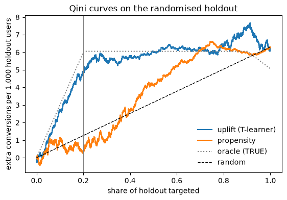

Out [9]:

Uplift sits well above the diagonal. Propensity hugs zero across the first quarter (loyalists), then dips as it reaches the sleeping dogs, then climbs once it finally hits the persuadables.

Honest note: over the whole curve the TRUE Qini of the propensity ranking is a little above random, because after the loyalists it does rank persuadables ahead of lost causes. Its observed Qini interval straddles zero. It loses to random where Northwind will actually buy media, the top 20%. Uplift beats random on both views.

6. The estimand beside the number

The registered E-USER-ITT reads “conversions per dollar for everyone assigned”. Maya’s number is conversions per 1,000 users targeted, over a 4-week flight, from a bootstrap. So she re-wraps it. Two things to know:

• intervention takes the spec’s shape (type, size, arms, population), not a free kind: target_top_k. “Target the top 20% of a ranking” goes in arms. Both rankings share it, which is what makes them comparable.
• metric_family cannot be passed as a keyword, and overriding kpi keeps the base’s sales_return. To set it explicitly, edit to_dict() and wrap again. Here it stays sales_return (conversions are sales), stated on purpose.

In [10]:

base = fin.estimand("E-USER-ITT", kpi="conversions_per_1000_users_targeted", per="absolute", channels="meta", weeks=4,
                    level=0.9, interval="bootstrap_pct",
                    intervention={"type": "remove_all", "size": -1.0, "size_kind": "relative",
                                  "arms": ["top_20pct_of_ranking", "holdout"], "population": "itt"})
try:
    fin.estimand("E-USER-ITT", metric_family="sales_return")
except TypeError as err:
    print("TypeError:", err)

d = base.to_dict()
d["metric_family"] = "sales_return"      # explicit, not inherited by accident
e = fin.estimand(d)
print(e.words, "|", e.spec.metric_family, "| registry id:", e.registry_id)

Out [10]:

TypeError: unknown estimand field(s) ['metric_family']; use one of: intervention, size, size_kind, arms, population, baseline, horizon, weeks, kpi, per, cost_basis, currency, point_rule, interval, level, channels, geos, client, scope_kpi
conversions per 1000 users targeted in total, net from removing all spend, itt, versus the control counterfactual, over 4 weeks, estimator point, 90% bootstrap_pct | sales_return | registry id: None

In [11]:

prop_n = fin.number(at_k.loc["propensity", "per_1000"], (at_k.loc["propensity", "lo_90"], at_k.loc["propensity", "hi_90"]),
                    e, label="propensity top 20%")
uplift_n = fin.number(at_k.loc["uplift (T-learner)", "per_1000"],
                      (at_k.loc["uplift (T-learner)", "lo_90"], at_k.loc["uplift (T-learner)", "hi_90"]),
                      e, label="uplift top 20%")
display(prop_n, uplift_n)
alignment = fin.compare(prop_n, uplift_n)
alignment

Out [11]:

propensity top 20%: 1.47

likely between -9.16 and 11.8 · low confidence

details

means	conversions per 1000 users targeted in total, net from removing all spend, itt, versus the control counterfactual, over 4 weeks, estimator point, 90% bootstrap_pct
interval	90% bootstrap_pct -9.16 to 11.81
trust level	2

uplift top 20%: 24.76

likely between 17.7 and 32.6 · medium confidence

details

means	conversions per 1000 users targeted in total, net from removing all spend, itt, versus the control counterfactual, over 4 weeks, estimator point, 90% bootstrap_pct
interval	90% bootstrap_pct 17.65 to 32.63
trust level	2

Same question

every field matches

details

why	all seven fields and scope match

fin.compare finds no field that differs: same population, intervention, horizon, unit and interval. The gap between the two numbers is the ranking, not a quiet change of question.

7. A Tier D audience manifest, labelled pilot

The planner needs one row per Meta line. Maya splits the uplift audience’s holdout readout into prospecting (no past orders) and retargeting (past buyers).

Where the contract runs out: a Tier D summary only takes metric="roi" or "mroi". The number sits under the roi label; the estimand says what it really is (conversions per 1,000 targeted).

In [12]:

prospect = (hold.past_orders == 0).to_numpy()


def line_readout(mask):
    idx = top_k(u_score)
    keep = idx[mask[idx]]
    yy, tt, ww = y[keep], t[keep], W[:, keep]
    est = lambda w: 1000 * ((w * yy * tt).sum(-1) / (w * tt).sum(-1) - (w * yy * (1 - tt)).sum(-1) / (w * (1 - tt)).sum(-1))
    lo, hi = np.percentile(est(ww), [5, 95])
    return est(np.ones(len(keep))), (lo, hi), len(keep), 1000 * tau_hold[keep].mean()


lines, line_n, line_ci, line_true = {}, {}, {}, {}
for name, mask in [("prospecting_meta", prospect), ("retargeting_meta", ~prospect)]:
    v, ci, n_top, truth = line_readout(mask)
    lines[name], line_n[name] = fin.number(v, ci, e, label=name), n_top
    line_ci[name], line_true[name] = ci, truth
    print(f"{name}: {v:.1f} per 1,000 targeted (90% {ci[0]:.1f} to {ci[1]:.1f}), n={n_top}; TRUE {truth:.1f}")

Out [12]:

prospecting_meta: 23.8 per 1,000 targeted (90% 15.8 to 32.2), n=8469; TRUE 28.1
retargeting_meta: 27.7 per 1,000 targeted (90% 10.6 to 43.0), n=3577; TRUE 11.8

Both intervals cover their TRUE values. Retargeting’s is wide (fewer users, higher base rates) and its TRUE is lower: the past buyers the uplift model lets in are partly loyalists. Worth saying out loud when the planner sees two rows.

First the manifest as most models arrive: no acceptance block, default capability.

In [13]:

m0 = fin.Model.from_table(lines, estimand=e, name="nw_hiker_uplift", engine="sklearn-two-model", family="audience",
                          metric="roi", dependence="declared_assumption")
m0.check().to_frame()[["gate", "outcome", "message"]]

Out [13]:

	gate	outcome	message
0	G-ACC-01	fallback	acceptance untested: usable, labelled unvalidated method, trust reduced
1	G-CAP-01	route	sandbox output: experimental label and a named approver needed

Both gates degrade instead of blocking: G-ACC-01 labels an unvalidated method, G-CAP-01 routes a sandbox model to an approver with an experimental label.

Why Maya runs the §16 checks herself: no gate is specific to the audience family. An audience model marked certified would pass G-CAP-01 without ever showing a randomised holdout. Spec §16 asks audience models for four things: declare uplift or propensity, validate uplift only on a randomised holdout, pass a known-truth simulation, and keep every segment above a minimum size. She checks them by hand and records them in acceptance. This notebook is the known-truth simulation: every readout above sat beside its TRUE value.

In [14]:

def covers(lo, hi, truth):
    return bool(lo <= truth <= hi)


known_truth = {                                                       # 90% intervals vs the TRUE values above
    "uplift_top20_covered": covers(*at_k.loc["uplift (T-learner)", ["lo_90", "hi_90", "TRUE"]]),
    **{f"{n}_covered": covers(*line_ci[n], line_true[n]) for n in lines},
    "scenarios": 1, "seed": SEED,
}
seg_floor = 50                                                        # G-PRIV-01 default, also used as the §16 floor
s16 = {
    "uplift_declared": True,                                          # the score is an uplift score, not a propensity
    "validated_on_randomised_holdout_only": not hold.index.isin(train.index).any(),   # treat was randomised per user
    "known_truth_simulation": all(v for k, v in known_truth.items() if k.endswith("_covered")),
    "min_segment_size": min(line_n.values()),                         # smallest holdout cell behind a reported line
}
assert all(s16.values()) and s16["min_segment_size"] >= seg_floor
s16

Out [14]:

{'uplift_declared': True,
 'validated_on_randomised_holdout_only': True,
 'known_truth_simulation': True,
 'min_segment_size': 3577}

In [15]:

m = fin.Model.from_table(
    lines, estimand=e, name="nw_hiker_uplift", engine="sklearn-two-model", family="audience", metric="roi",
    dependence="declared_assumption", capability_status="pilot",
    acceptance={"status": "pilot",
                "identification": {"status": "untested", "metrics": {"section_16": s16, "known_truth": known_truth}},
                "decisions": {"status": "untested",
                              "metrics": {"qini_uplift": round(float(qini_table.loc["uplift (T-learner)", "Qini"]), 3),
                                          "qini_propensity": round(float(qini_table.loc["propensity", "Qini"]), 3)}}},
    notes=[{"text": "Tier D: value is incremental conversions per 1,000 targeted (see estimand), stored under roi"},
           {"text": "dependence declared_assumption: lines share one holdout bootstrap; not joint draws"}],
)
report = m.check()
display(m)
report.to_frame()[["gate", "outcome", "message"]]

Out [15]:

nw_hiker_uplift · Tier D

2 channels, audience

details

engine	sklearn-two-model
dependence	declared_assumption
acceptance	pilot
estimands	roi: custom

channel	value	lo	hi	level	current_spend
prospecting_meta	23.79	15.815	32.175	0.9	None
retargeting_meta	27.75	10.591	42.969	0.9	None

	gate	outcome	message
0	G-ACC-01	fallback	acceptance pilot: usable, labelled unvalidated method, trust reduced

With capability_status="pilot", G-CAP-01 passes. G-ACC-01 still fires: a pilot acceptance is usable but labelled, trust reduced by one. That is the right label for a first audience model.

Why identification stays untested though the simulation recovered the truth: it is one scenario on one seed, with no pass mark set. The §14 identification layer wants a battery of known-truth scenarios; this run is recorded as evidence toward it, not as the bar.

8. Releasing the segments: a privacy stop

Meta gets the audience as named segments. Maya scores all 200,000 users, takes the top 20% and cuts it the way the media team asked. Every release names its destination, its segment sizes and the aggregate behind them: the privacy gates fail closed on a release that leaves any of them out.

In [16]:

users["u_score"] = uplift_score(users)
audience = users.loc[top_k(users.u_score.to_numpy())]
age_band = pd.cut(audience.age, [0, 24, 34, 54, 200], labels=["18_24", "25_34", "35_54", "55_plus"])
cell = np.where(audience.climber == 1, np.where(audience.rural == 1, "climbers_rural", "climbers_urban"),
                "hikers_" + age_band.astype(str))
segments = pd.Series(cell).value_counts().rename_axis("id").rename("size").reset_index()
segments

Out [16]:

	id	size
0	hikers_35_54	17818
1	hikers_25_34	13839
2	hikers_18_24	5978
3	hikers_55_plus	2067
4	climbers_urban	256
5	climbers_rural	42

In [17]:

def release(segs):
    # A release states where it goes, its cell sizes and the aggregate behind them; leave one out and it fails closed.
    return fin.check("model_manifest", m.doc, operation="audience_output",
                     context={"destination": "export",                      # Meta, outside UMP
                              "segments": segs.to_dict("records"),
                              "aggregate": {"query": "top 20% by uplift score, cut by segment",
                                            "n": int(segs["size"].sum())}})


r = release(segments)
try:
    r.raise_for_stops()
except fin.Stopped as stop:
    print(stop.code, "|", stop.gate, "|", stop.detail)

Out [17]:

PRIVACY_FLOOR | G-PRIV-01 | G-PRIV-01: 1 segment(s) below minimum size 50

A hard stop. A segment that small can single out people, and G-PRIV-01 is one of the eight gates that never degrade. Maya merges the two climber cells and checks again.

In [18]:

merged = segments.assign(id=segments.id.replace({"climbers_rural": "climbers", "climbers_urban": "climbers"}))
merged = merged.groupby("id", as_index=False)["size"].sum()
r2 = release(merged)
r2.raise_for_stops()
print("ok:", r2.ok, "| smallest segment:", merged["size"].min())
r2.to_frame()[["gate", "outcome", "message"]]

Out [18]:

ok: True | smallest segment: 298

	gate	outcome	message
0	G-ACC-01	fallback	acceptance pilot: usable, labelled unvalidated method, trust reduced

Summary

• Asked: prove a “high-value hikers” audience beats broad targeting on Meta.
• Handed over: the uplift audience adds the number below, with its estimand and interval. The propensity audience, on the same estimand, adds about nothing.
• Assumed or fell back: G-ACC-01 labels the model unvalidated (pilot acceptance); the two Meta lines carry a declared dependence assumption, not joint draws; the value sits under the roi label of a Tier D summary; climbers_rural was merged into climbers after the G-PRIV-01 stop.
• Next: a second randomised flight that targets the top 20% and holds out a slice of it, so the audience earns its own readout before anyone calls it certified.

In [19]:

handover = uplift_n
print(handover, "|", handover.estimand.words)
print(f"TRUE oracle {TRUE['oracle_at_k']:.0f}, TRUE value of this ranking {at_k.loc['uplift (T-learner)', 'TRUE']:.1f}, "
      f"random {TRUE['random_at_k']:.0f} per 1,000 targeted")

Out [19]:

<Number uplift top 20%: 24.76 (90% 17.65 to 32.63)> | conversions per 1000 users targeted in total, net from removing all spend, itt, versus the control counterfactual, over 4 weeks, estimator point, 90% bootstrap_pct
TRUE oracle 30, TRUE value of this ranking 23.3, random 5 per 1,000 targeted

Going deeper

• Sweep K: uplift@k falls as the audience grows past the persuadables; the Qini curve shows where.
• Swap the T-learner for an X-learner or a transformed-outcome model; the readout code does not change.
• Notebook 01 covers fin.compare when two estimands do differ; notebook 02 covers the gates and strict mode.

Next: notebook 11 reads a user-level conversion-lift test (ITT and CACE) with the same E-USER-ITT estimand.