15 · Forecasting the Q3 plan, judged on weeks it never saw

You will learn

Backtest a forecast on held-out weeks and read its interval coverage
Spot a plan that leaves the history the model was fitted on
Add scenario uncertainty instead of shipping a point forecast
File a forecaster as a Tier D model and see what stays pilot

You need

Python 3.12 and uv

Run this notebook Offline

notebooks/15_forecasting_a_plan_on_held_out_weeks.ipynb

Runs offline on your laptop. The outputs on this page were saved from a real run.

About 25 minutes

Access needed. The packages and notebooks are not yet publicly distributed. The steps below need a checkout of the UMP repository. Pages show recorded outputs, so you can follow along without running them.

cd notebooks && uv run jupyter lab

Runs offline. Uses babelfin and scikit-learn. The data is SYNTHETIC, generated below with a known truth.

Northwind Outdoor wants one number by Thursday: Q3 sales if they run the new plan. Sam Patel has MMM curves, so his first draft is quick. Push the plan through the curves, add up thirteen weeks, done. Two things should worry him. The interval only knows about the model’s own fit, and the plan puts CTV 60% above any week Northwind has ever bought. This notebook checks the forecast on weeks it never saw, finds it overconfident, and fixes the interval before it goes out.

In [1]:

import babelfin as fin
import matplotlib.pyplot as plt
import numpy as np
import pandas as pd
from sklearn.linear_model import Ridge
from sklearn.pipeline import make_pipeline
from sklearn.preprocessing import StandardScaler

SEED = 24
CH = ["tv", "ctv", "search"]
pd.set_option("display.max_colwidth", None)   # an estimand is a sentence; never cut it short


def table(numbers):
    """fin.Numbers as rows: value, interval and the estimand in words."""
    return pd.DataFrame([{"number": k, "value": round(n.value), "lo": round(n.lo), "hi": round(n.hi),
                          "estimand": n.estimand.words} for k, n in numbers.items()])

1. “What will Q3 be?”

The ask, as the client wrote it: Q3 sales if we run this plan, and how that compares with business as usual. Thirteen weeks, two spend plans, one answer each. A point line would be easy to draw. The rest of the notebook is about the band around it.

2. A synthetic history, and a plan that leaves it

Three years of weekly sales: trend, yearly seasonality, three channels with carryover (adstock) and Hill saturation, and a demand index (think consumer confidence) that wanders and takes a sharp hit in week 149. Spend is booked in advance and delivered within ±15%, as it is in real life. TRUE holds everything the forecast should recover.

In [2]:

TRUE = {"weeks": 156, "q3_weeks": 13, "base": 100_000.0, "trend_per_week": 120.0, "season_amp": 0.18,
        "noise_sd": 3_000.0, "demand_beta": 60_000.0, "demand_phi": 0.9, "demand_sd": 0.03,
        "shock": {"week": 149, "size": -0.25}, "delivery_sd": 0.075,
        "channels": {"tv": {"beta": 38_000.0, "half_life": 3, "k": 60_000.0, "s": 1.4},
                     "ctv": {"beta": 34_000.0, "half_life": 2, "k": 12_000.0, "s": 1.6},
                     "search": {"beta": 26_000.0, "half_life": 1, "k": 12_000.0, "s": 1.2}}}
T, H = TRUE["weeks"], TRUE["q3_weeks"]


def decay(half_life):
    return 0.5 ** (1 / half_life)


def adstock(x, d):
    out = np.zeros(len(x))
    for t, v in enumerate(x):
        out[t] = v + (d * out[t - 1] if t else 0.0)
    return out * (1 - d)


def hill(a, k, s):
    return a**s / (a**s + k**s)


def demand_path(rng, n, start=0.0, t0=0, shock=True):
    x, out = start, np.zeros(n)
    for i in range(n):
        hit = TRUE["shock"]["size"] if shock and t0 + i == TRUE["shock"]["week"] else 0.0
        x = TRUE["demand_phi"] * x + rng.normal(0, TRUE["demand_sd"]) + hit
        out[i] = x
    return out


def true_sales(t, spend, demand):
    """Expected sales under the true process (no noise)."""
    season = np.sin(2 * np.pi * t / 52) + 0.4 * np.cos(4 * np.pi * t / 52)
    base = (TRUE["base"] + TRUE["trend_per_week"] * t) * (1 + TRUE["season_amp"] * season)
    media = sum(c["beta"] * hill(adstock(spend[ch].to_numpy(), decay(c["half_life"])), c["k"], c["s"])
                for ch, c in TRUE["channels"].items())
    return base + TRUE["demand_beta"] * demand + media


def deliver(booked, rng):
    return booked * np.clip(1 + rng.normal(0, TRUE["delivery_sd"], booked.shape), 0.85, 1.15)


rng = np.random.default_rng(SEED)
t_hist = np.arange(T)
booked = pd.DataFrame({"tv": rng.gamma(6, 10_000, T), "ctv": rng.gamma(5, 3_000, T), "search": rng.gamma(8, 1_500, T)})
delivered = deliver(booked, rng)
demand = demand_path(rng, T)
hist = pd.DataFrame({"t": t_hist, **delivered, **booked.add_suffix("_booked"), "demand_index": demand})
hist["sales"] = true_sales(t_hist, delivered, demand) + rng.normal(0, TRUE["noise_sd"], T)
hist[["sales", *CH, "demand_index"]].describe().round(2)

Out [2]:

	sales	tv	ctv	search	demand_index
count	156.00	156.00	156.00	156.00	156.00
mean	158787.89	56717.86	16138.43	11909.66	-0.02
std	14652.14	24437.61	7208.84	4430.50	0.05
min	124639.42	12524.02	3438.80	2427.89	-0.17
25%	146957.64	36921.63	10786.72	8318.76	-0.05
50%	161080.22	54883.14	15459.17	11506.59	-0.02
75%	170455.19	71473.70	20489.81	15044.04	0.02
max	192346.74	131803.12	41355.77	24486.08	0.10

The Q3 plan cuts TV by 15%, adds 10% to search and pushes CTV hard: ten of the thirteen weeks sit above the most CTV Northwind has ever delivered in a week, peaking at 1.6 times it. BAU repeats last year’s average week.

The true Q3 is simulated forward under each plan with fresh noise, one future, the same for both plans. It stays in TRUE and the forecast never reads it.

In [3]:

t_q3 = np.arange(T, T + H)
bau = pd.DataFrame({c: np.full(H, booked[c].iloc[-52:].mean()) for c in CH})
plan = bau.assign(tv=bau.tv * 0.85, search=bau.search * 1.10,
                  ctv=np.r_[np.full(3, bau.ctv.iloc[0] * 1.5), np.full(10, delivered.ctv.max() * 1.6)])

fut = np.random.default_rng(SEED + 100)                     # the one future that actually happens
q3_demand = demand_path(fut, H, start=demand[-1], t0=T, shock=False)
q3_mult = np.clip(1 + fut.normal(0, TRUE["delivery_sd"], (H, 3)), 0.85, 1.15)
q3_noise = fut.normal(0, TRUE["noise_sd"], H)
t_all, dem_all = np.r_[t_hist, t_q3], np.r_[demand, q3_demand]
for name, p in [("plan", plan), ("bau", bau)]:
    spend = pd.concat([delivered, p * q3_mult], ignore_index=True)
    TRUE[f"q3_{name}_sales_true"] = float((true_sales(t_all, spend, dem_all)[T:] + q3_noise).sum())
TRUE["q3_diff_true"] = TRUE["q3_plan_sales_true"] - TRUE["q3_bau_sales_true"]
TRUE["ctv_plan_vs_hist_max"] = round(plan.ctv.max() / delivered.ctv.max(), 2)
print("CTV plan peak vs historical max:", TRUE["ctv_plan_vs_hist_max"])
print("weeks with CTV above the historical max:", int((plan.ctv > delivered.ctv.max()).sum()), "of", H)

Out [3]:

CTV plan peak vs historical max: 1.6
weeks with CTV above the historical max: 10 of 13

In [4]:

fig, ax = plt.subplots(figsize=(9, 2.6))
ax.plot(t_hist, delivered.ctv, color="grey", lw=1, label="CTV delivered (history)")
ax.plot(t_q3, plan.ctv, color="C3", lw=2, label="CTV in the Q3 plan")
ax.axhline(delivered.ctv.max(), ls=":", color="k", lw=1, label="historical max")
ax.set_xlabel("week"); ax.set_ylabel("USD per week"); ax.legend(loc="upper left", fontsize=8)
plt.show()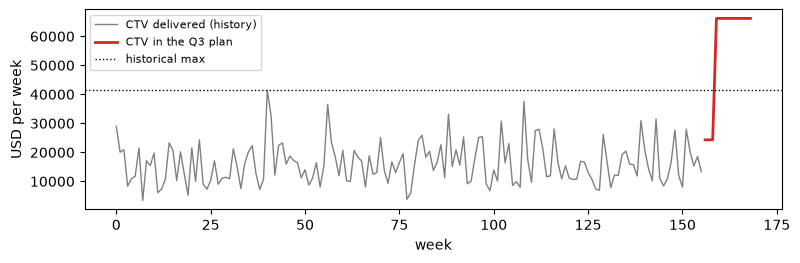

Out [4]:

CTV spend in USD per week. The delivered history, weeks 0 to 155, moves between about 5,000 and 41,000, with a dotted line at the historical maximum near 41,000. The Q3 plan in red starts near 24,000 and jumps to about 66,000, well above anything in the history.

3. Sam’s first draft

The forecaster is a ridge regression on adstocked, log-saturated media plus trend and two Fourier pairs of seasonality. Half-lives come from a small grid, scored on weeks 105 to 144. The interval is a residual bootstrap: refit on resampled residuals, then add a resampled residual to each forecast week. That captures the fit’s own uncertainty and ordinary week-to-week noise. It knows nothing about the scenario: the plan is taken as delivered exactly and demand is ignored.

In [5]:

def features(spend, t, half_lives, scale, demand=None):
    cols = {c: np.log1p(adstock(spend[c].to_numpy(), decay(half_lives[c])) / scale[c]) for c in CH}
    cols["trend"] = t / 52
    for k in (1, 2):
        cols[f"sin{k}"], cols[f"cos{k}"] = np.sin(2 * np.pi * k * t / 52), np.cos(2 * np.pi * k * t / 52)
    if demand is not None:
        cols["demand"] = demand
    return pd.DataFrame(cols)


def ridge():
    return make_pipeline(StandardScaler(), Ridge(alpha=1.0))


def pick_half_lives(train):
    scale, best = {c: train[c].mean() for c in CH}, None
    for hl in [(a, b, c) for a in range(1, 5) for b in range(1, 5) for c in range(1, 5)]:
        X = features(train[CH], train.t.to_numpy(), dict(zip(CH, hl)), scale)
        err = np.mean((ridge().fit(X[:104], train.sales[:104]).predict(X[104:144]) - train.sales[104:144]) ** 2)
        best = min(best or (err, hl), (err, hl))
    return dict(zip(CH, best[1]))


def fit(train, half_lives, use_demand, n_boot=200, seed=0):
    """Ridge fit plus a residual bootstrap: n_boot refits, each on fitted + resampled residuals."""
    scale = {c: train[c].mean() for c in CH}
    X = features(train[CH], train.t.to_numpy(), half_lives, scale, train.demand_index.to_numpy() if use_demand else None)
    y = train.sales.to_numpy()
    m = ridge().fit(X, y)
    fitted, r = m.predict(X), np.random.default_rng(seed)
    res = y - fitted
    boots = [ridge().fit(X, fitted + r.choice(res, len(y))) for _ in range(n_boot)]
    return {"model": m, "boots": boots, "res": res, "scale": scale, "half_lives": half_lives,
            "use_demand": use_demand, "demand": train.demand_index.to_numpy(),
            "cap_ctv": X["ctv"].max()}


HL = pick_half_lives(hist)
draft = fit(hist, HL, use_demand=False, seed=1)
print("half-lives picked:", HL)

Out [5]:

half-lives picked: {'tv': 4, 'ctv': 3, 'search': 1}

In [6]:

def draft_draws(F, past_spend, future_spend, t_future, seed):
    """Parameter + noise only: booked spend taken as delivered, demand ignored."""
    r, n = np.random.default_rng(seed), len(future_spend)
    spend = pd.concat([past_spend, future_spend], ignore_index=True)
    t = np.r_[np.arange(len(past_spend)), t_future]
    X = features(spend, t, F["half_lives"], F["scale"]).iloc[-n:]
    return np.array([b.predict(X) + r.choice(F["res"], n) for b in F["boots"]])


q3_draft = draft_draws(draft, delivered, plan, t_q3, seed=2).sum(axis=1)
f_level = fin.estimand("E-MMM-ROI", kpi="sales", per="absolute", intervention={"type": "scale", "arms": ["q3_plan"]},
                       baseline="current_plan", weeks=13, level=0.9, point_rule="posterior_median",
                       interval="bootstrap_pct")
first_draft = fin.number(np.median(q3_draft), tuple(np.quantile(q3_draft, [0.05, 0.95])), f_level,
                         label="Q3 sales under the plan (first draft)")
first_draft

Out [6]:

Q3 sales under the plan (first draft): 2,605,620

likely between $2.5M and $2.7M · medium confidence

details

means	sales in total, net from scaling spend, versus the current plan, over 13 weeks, posterior median, 90% bootstrap_pct
interval	90% bootstrap_pct 2,547,470 to 2,665,060
trust level	2

4. The setback: twelve weeks it never saw

Before this goes to the client, Sam backtests it. For each of the last twelve weeks of history (144 to 155) he refits on the weeks before it and forecasts that week from the spend that was booked, one week ahead. Two checks from spec §16 for forecasting models:

Coverage. A 90% interval should contain about 11 of the 12 actual weeks.
Beats naive. MASE scales the error by the in-sample error of a seasonal-naive forecast (same week last year). Below 1 beats it; the naive forecast’s own MASE on the same weeks is the bar to clear.

In [7]:

HOLD = list(range(T - 12, T))
y_in = hist.sales.to_numpy()[: T - 12]
NAIVE_SCALE = np.mean(np.abs(y_in[52:] - y_in[:-52]))   # in-sample seasonal-naive MAE
BOOKED = hist[[f"{c}_booked" for c in CH]].set_axis(CH, axis=1)


def backtest(method):
    rows = []
    for w in HOLD:
        train = hist.iloc[:w]
        F = fit(train, HL, use_demand=(method == "fixed"), seed=w)
        draws = method_draws[method](F, train[CH], BOOKED.iloc[[w]].reset_index(drop=True), np.array([w]), seed=1000 + w)
        lo, hi = np.quantile(draws[:, 0], [0.05, 0.95])
        rows.append({"week": w, "actual": hist.sales[w], "forecast": np.median(draws[:, 0]), "lo": lo, "hi": hi,
                     "seasonal_naive": hist.sales[w - 52]})
    df = pd.DataFrame(rows).assign(covered=lambda d: (d.lo <= d.actual) & (d.actual <= d.hi))
    score = {"coverage": df.covered.mean(), "MASE": np.mean(np.abs(df.actual - df.forecast)) / NAIVE_SCALE,
             "MASE_seasonal_naive": np.mean(np.abs(df.actual - df.seasonal_naive)) / NAIVE_SCALE}
    return df, {k: round(float(v), 3) for k, v in score.items()}


method_draws = {"draft": draft_draws}
bt_draft, score_draft = backtest("draft")
print(score_draft)
bt_draft.round(0)

Out [7]:

{'coverage': 0.583, 'MASE': 0.544, 'MASE_seasonal_naive': 0.653}

	week	actual	forecast	lo	hi	seasonal_naive	covered
0	144	149069.0	143116.0	138656.0	149786.0	142339.0	True
1	145	142851.0	142203.0	135605.0	148108.0	135199.0	True
2	146	146787.0	142375.0	136614.0	148532.0	144035.0	True
3	147	150602.0	147819.0	142359.0	154421.0	138290.0	True
4	148	160155.0	153659.0	147789.0	159566.0	143273.0	False
5	149	144328.0	154376.0	148340.0	160319.0	148038.0	False
6	150	149066.0	155530.0	149176.0	161953.0	156778.0	False
7	151	153441.0	161057.0	155561.0	166449.0	153344.0	False
8	152	165076.0	165103.0	159072.0	171822.0	161965.0	True
9	153	161217.0	167884.0	161513.0	172878.0	156986.0	False
10	154	167776.0	172210.0	164875.0	178338.0	168784.0	True
11	155	172441.0	173606.0	167232.0	178648.0	170523.0	True

Seven of twelve weeks covered: 58% from an interval that calls itself 90%. Four of the five misses sit around week 149, when demand dropped and the draft had no way to know. MASE does beat seasonal naive (0.54 against 0.65), by less than a fifth. On Thursday this interval would have been reported as 90% and behaved like a coin with a slight lean.

5. The fix: say what the forecast does not know

Sam adds three things. Each one is an assumption, and the notebook names it as one.

Demand is in the model, and its future is a scenario. The demand index joins the regressors. Its future is drawn as an AR(1) from its last value. The persistence is drawn between 0.75 and 0.95 (the fitted value sits near 0.8; the planning team expects shocks to fade more slowly).
Delivery is a scenario. Each draw delivers the booked plan within ±15%, the range seen in history.
CTV beyond history is widened. Where adstocked CTV exceeds its historical maximum, the extra response is drawn between nothing (flat at the edge of the data) and what the fitted curve says. No data can tell those apart, so the interval spans both. The backtest cannot test this piece because no held-out week leaves the historical range.

Plan and BAU use the same random numbers, so their difference keeps only what the plans change.

In [8]:

ASSUMPTIONS = {
    "demand_scenario": "AR(1) from the last observed demand index; persistence ~ Uniform(0.75, 0.95)",
    "delivery_scenario": "delivered = booked x (1 + N(0, 0.075)), clipped to +-15%",
    "extrapolation": "CTV response above the historical max adstock ~ Uniform(0, 1) x the fitted curve's increment",
    "noise": "residuals resampled as one contiguous block, so serial correlation carries into multi-week sums",
}


def scenario_draws(F, past_spend, future_spend, t_future, seed, widen=True):
    """Parameter + noise + demand and delivery scenarios + extrapolation widening (all labelled above)."""
    r, n = np.random.default_rng(seed), len(future_spend)
    d = F["demand"]
    sd = np.std(d[1:] - np.corrcoef(d[:-1], d[1:])[0, 1] * d[:-1])
    t = np.r_[np.arange(len(past_spend)), t_future]
    out = []
    for b in F["boots"]:
        mult = np.clip(1 + r.normal(0, 0.075, (n, 3)), 0.85, 1.15)
        phi, x, dem = r.uniform(0.75, 0.95), d[-1], []
        for _ in range(n):
            x = phi * x + r.normal(0, sd)
            dem.append(x)
        start = r.integers(0, len(F["res"]) - n + 1)
        u = r.uniform() if widen else 1.0
        spend = pd.concat([past_spend, future_spend * mult], ignore_index=True)
        X = features(spend, t, F["half_lives"], F["scale"], np.r_[d, dem]).iloc[-n:]
        over = np.maximum(X["ctv"] - F["cap_ctv"], 0.0)
        X = X.assign(ctv=X["ctv"] - over + u * over)
        out.append(b.predict(X) + F["res"][start:start + n])
    return np.array(out)


method_draws["fixed"] = scenario_draws

6. Backtest again

In [9]:

bt_fixed, score_fixed = backtest("fixed")
print("missed weeks:", bt_fixed.week[~bt_fixed.covered].tolist())
pd.DataFrame({"first draft": score_draft, "with scenarios": score_fixed}).T

Out [9]:

missed weeks: [149]

	coverage	MASE	MASE_seasonal_naive
first draft	0.583	0.544	0.653
with scenarios	0.917	0.406	0.653

In [10]:

fig, ax = plt.subplots(figsize=(9, 3))
for df, name, off, col in [(bt_draft, "first draft", -0.15, "C0"), (bt_fixed, "with scenarios", 0.15, "C2")]:
    ax.vlines(df.week + off, df.lo, df.hi, color=col, lw=3, alpha=0.6, label=f"{name} 90% interval")
ax.plot(bt_fixed.week, bt_fixed.actual, "k.", ms=9, label="actual")
ax.axvline(TRUE["shock"]["week"] - 0.5, ls=":", color="grey")
ax.set_xlabel("held-out week"); ax.set_ylabel("sales"); ax.legend(fontsize=8, loc="upper left")
plt.show()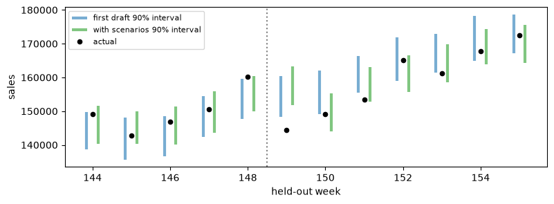

Out [10]:

Sales for held-out weeks 144 to 155: for each week a blue first-draft 90% interval, a green interval with scenarios, and a black dot for the actual. After week 148 the actuals start to fall outside the first-draft intervals, for example week 149 at about 144,000. The wider green intervals cover more of them.

Eleven of twelve: 92% coverage on a 90% interval, and MASE now clearly beats seasonal naive. The one miss is week 149 itself, the shock no forecast made the week before could see.

Why only twelve weeks? Sam picked it to match one quarter; spec §16 names held-out periods but sets no window length. Twelve is small, though: each week moves coverage by eight points. One week ahead is also shorter than the thirteen-week Q3 horizon, so the backtest checks the method, not the horizon. Both limits go in the handover.

7. Plan versus BAU, as numbers with estimands

The final fit uses all 156 weeks and 400 bootstrap refits. The estimand comes from E-MMM-ROI with every field set for this question: sales in USD over 13 weeks, posterior median, 90% bootstrap interval, the plan as a scenario against the current plan.

A gap worth knowing. fin.estimand has no metric_family keyword, and overriding kpi keeps the base’s sales_return. The fix is to edit the dict and wrap it again. The words still say “versus the current plan” on the level numbers; read them as sales under the scenario the arm names.

In [11]:

def with_family(e, family):
    d = e.to_dict()
    d["metric_family"] = family
    return fin.estimand(d)


f = with_family(f_level, "sales_forecast")
f_bau = with_family(fin.estimand(f, intervention={"type": "scale", "size": 0.0, "arms": ["bau_plan"]}), "sales_forecast")
f_diff = with_family(fin.estimand(f, kpi="incremental_sales"), "sales_forecast")
print(f.words, "|", f.to_dict()["metric_family"])

Out [11]:

sales in total, net from scaling spend, versus the current plan, over 13 weeks, posterior median, 90% bootstrap_pct | sales_forecast

In [12]:

final = fit(hist, HL, use_demand=True, n_boot=400, seed=7)
plan_w = scenario_draws(final, delivered, plan, t_q3, seed=99)                 # weekly draws, 400 x 13
bau_w = scenario_draws(final, delivered, bau, t_q3, seed=99)                   # same random numbers: paired
plan_raw = scenario_draws(final, delivered, plan, t_q3, seed=99, widen=False)  # no extrapolation widening


def shown(draws, est, label):
    return fin.number(np.median(draws), tuple(np.quantile(draws, [0.05, 0.95])), est, label=label)


plan_n = shown(plan_w.sum(axis=1), f, "Q3 sales, plan")
bau_n = shown(bau_w.sum(axis=1), f_bau, "Q3 sales, BAU")
diff_n = shown(plan_w.sum(axis=1) - bau_w.sum(axis=1), f_diff, "Q3 plan minus BAU")
plan_unwidened = shown(plan_raw.sum(axis=1), f, "Q3 sales, plan, without the widening")
table({"plan": plan_n, "bau": bau_n, "plan minus bau": diff_n, "plan, not widened": plan_unwidened})

Out [12]:

	number	value	lo	hi	estimand
0	plan	2446734	2373736	2529812	sales in total, net from scaling spend, versus the current plan, over 13 weeks, posterior median, 90% bootstrap_pct
1	bau	2355183	2298968	2403663	sales in total, net from scaling spend (+0%), versus the current plan, over 13 weeks, posterior median, 90% bootstrap_pct
2	plan minus bau	90971	36276	170178	incremental sales in total, net from scaling spend, versus the current plan, over 13 weeks, posterior median, 90% bootstrap_pct
3	plan, not widened	2518115	2442253	2587038	sales in total, net from scaling spend, versus the current plan, over 13 weeks, posterior median, 90% bootstrap_pct

Months add up to the quarter

Sales in USD (per="absolute") are additive, so monthly numbers can be summed. fin.total does not check that for you: it would add ratios just as happily. Given the months as separate numbers it cannot know how they move together, so it takes the G-DEP-01 envelope. Given the joint draws, it adds draw by draw.

In [13]:

months = {"jul": slice(0, 4), "aug": slice(4, 8), "sep": slice(8, 13)}
monthly = {m: shown(plan_w[:, s].sum(axis=1), fin.estimand(f, weeks=s.stop - s.start), f"plan, {m}")
           for m, s in months.items()}
envelope = fin.total(monthly)
joint = fin.total(pd.DataFrame({m: plan_w[:, s].sum(axis=1) for m, s in months.items()}))
print("from three shown numbers:", envelope)
print("from the joint draws:    ", joint)

Out [13]:

from three shown numbers: <Total 2,451,424 (2,361,949 to 2,547,322, per_channel_envelope)>
from the joint draws:     <Total 2,446,734 (2,373,736 to 2,529,812, joint_draws)>

In [14]:

alignment = fin.compare(plan_n, bau_n)
print(alignment, "| mismatched:", alignment.mismatched)

Out [14]:

<Alignment assumed_alignment; differs on intervention> | mismatched: ['intervention']

Plan and BAU differ only on intervention, which is the point of the comparison. Horizon, unit, point rule and interval all match, so the difference is a like-for-like number.

Against the truth

In [15]:

truth = pd.DataFrame([
    {"number": n.label, "lo": round(n.lo), "hi": round(n.hi), "truth": round(TRUE[k])}
    for n, k in [(plan_n, "q3_plan_sales_true"), (bau_n, "q3_bau_sales_true"), (diff_n, "q3_diff_true"),
                 (plan_unwidened, "q3_plan_sales_true"), (first_draft, "q3_plan_sales_true")]])
truth["covered"] = (truth.lo <= truth.truth) & (truth.truth <= truth.hi)
truth

Out [15]:

	number	lo	hi	truth	covered
0	Q3 sales, plan	2373736	2529812	2419016	True
1	Q3 sales, BAU	2298968	2403663	2322789	True
2	Q3 plan minus BAU	36276	170178	96228	True
3	Q3 sales, plan, without the widening	2442253	2587038	2419016	False
4	Q3 sales under the plan (first draft)	2547470	2665060	2419016	False

The handed-over plan, BAU and difference intervals all contain the true Q3. The two that leave something out do not: the first draft and the plan without widening both sit above the truth. Their fitted log curve kept rising past the data while the true Hill curve flattened. The widening is what saved the plan number. One future is still only one future, so treat this as evidence for the method.

8. Filing the forecaster as a Tier D model

No Tier D shape exists for forecasts. A Tier D summary row only takes metric="roi" or "mroi". So the per-channel Q3 numbers sit under roi, and the estimand carries what they mean: incremental sales in USD from each channel’s change in the plan, plan minus BAU, over 13 weeks. The model is linear in its features, so the channel rows add up to the plan-minus-BAU number.

In [16]:

def channel_deltas(F, seed=99):
    """Per-channel Q3 incremental sales, plan minus BAU, from the same paired draws (widened CTV)."""
    out = {}
    for c in CH:
        mixed = bau.assign(**{c: plan[c]})
        out[c] = (scenario_draws(F, delivered, mixed, t_q3, seed) - bau_w).sum(axis=1)
    return out


deltas = channel_deltas(final)
by_channel = {c: shown(v, f_diff, f"{c}: plan minus BAU") for c, v in deltas.items()}
print("channels add up to the total:", np.allclose(sum(deltas.values()), plan_w.sum(axis=1) - bau_w.sum(axis=1)))
table(by_channel)

Out [16]:

channels add up to the total: True

	number	value	lo	hi	estimand
0	tv	-16313	-20665	-12145	incremental sales in total, net from scaling spend, versus the current plan, over 13 weeks, posterior median, 90% bootstrap_pct
1	ctv	99310	44905	177181	incremental sales in total, net from scaling spend, versus the current plan, over 13 weeks, posterior median, 90% bootstrap_pct
2	search	9438	7525	11548	incremental sales in total, net from scaling spend, versus the current plan, over 13 weeks, posterior median, 90% bootstrap_pct

In [17]:

widening = round((plan_n.hi - plan_n.lo) / (plan_unwidened.hi - plan_unwidened.lo), 2)
NOTES = [{"code": "EXTRAPOLATION_ASSUMED",
          "text": f"CTV plan reaches {TRUE['ctv_plan_vs_hist_max']}x the historical weekly max; response above the "
                  f"historical max adstock drawn between flat and the fitted curve; Q3 plan interval widened "
                  f"{widening}x", "widening_factor": widening},
         {"code": "SCENARIO_UNCERTAINTY", "text": "; ".join(f"{k}: {v}" for k, v in ASSUMPTIONS.items())},
         {"code": "KPI_UNDER_ROI_LABEL", "text": "no Tier D shape for forecasts: incremental USD sales sit under 'roi'"}]

m = fin.Model.from_table(by_channel, estimand=f_diff, name="nw_q3_forecast", engine="ridge-adstock",
                         family="forecasting", dependence="joint_draws", notes=NOTES)
print("widening factor on the Q3 plan interval:", widening)
m.check().to_frame()

Out [17]:

widening factor on the Q3 plan interval: 1.08

	gate	outcome	message	codes
0	G-ACC-01	fallback	acceptance untested: usable, labelled unvalidated method, trust reduced	UNVALIDATED_METHOD
1	G-CAP-01	route	sandbox output: experimental label and a named approver needed	EXPERIMENTAL_LABEL

Two gates fire, neither blocks. G-ACC-01 labels the method unvalidated: there is no acceptance record. G-CAP-01 labels the output experimental because a new model defaults to sandbox. No gate knows the §16 forecasting checks, so Sam records his hand-run ones in the acceptance block and moves the model to pilot.

In [18]:

ACCEPTANCE = {"status": "pilot",
              "decisions": {"status": "passed",
                            "metrics": {"check": "spec §16 forecasting, hand-run in this notebook",
                                        "held_out_weeks": 12, "lead_weeks": 1,
                                        "coverage_90": score_fixed["coverage"], "coverage_target": "0.88 to 0.92 (proposed)",
                                        "mase": score_fixed["MASE"], "mase_seasonal_naive": score_fixed["MASE_seasonal_naive"],
                                        "beats_naive": score_fixed["MASE"] < min(1.0, score_fixed["MASE_seasonal_naive"])}}}
m = fin.Model.from_table(by_channel, estimand=f_diff, name="nw_q3_forecast", engine="ridge-adstock",
                         family="forecasting", dependence="joint_draws", notes=NOTES,
                         acceptance=ACCEPTANCE, capability_status="pilot")
report = m.check()
print(report)
report.to_frame()

Out [18]:

<GateReport Would pass · 0 stops · 1 fallbacks · 0 warnings · 14 gates (1 fired)>

	gate	outcome	message	codes
0	G-ACC-01	fallback	acceptance pilot: usable, labelled unvalidated method, trust reduced	UNVALIDATED_METHOD

G-CAP-01 is gone. G-ACC-01 stays, now reading acceptance pilot. That is right: hand-run checks in a notebook are not a validated acceptance report, and only a linked one clears the gate. Claiming "passed" without one does not help either; the gate calls it ACCEPTANCE_UNSUBSTANTIATED.

strict=True turns that fallback into a stop, for a run where an unvalidated forecaster must not reach a client.

In [19]:

strict = m.check(strict=True)
print(strict)
try:
    strict.raise_for_stops()
except fin.Stopped as stop:
    print("stopped:", stop.code)

Out [19]:

<GateReport Stopped · 1 stops · 0 fallbacks · 0 warnings · 14 gates (1 fired)>
stopped: UNVALIDATED_METHOD

9. What Sam hands over

Asked: Q3 sales if Northwind runs the new plan, against business as usual.

Handed over (estimand: sales in USD over the 13 Q3 weeks, posterior median, 90% bootstrap interval):

In [20]:

print(f"Q3 sales, plan:     {plan_n}")
print(f"Q3 sales, BAU:      {bau_n}")
print(f"Plan minus BAU:     {diff_n}")
print(f"estimand: {diff_n.estimand.words}")
print(f"Backtest (12 held-out weeks, 1 week ahead): coverage {score_fixed['coverage']:.0%} of a 90% interval, "
      f"MASE {score_fixed['MASE']} vs seasonal naive {score_fixed['MASE_seasonal_naive']}")

Out [20]:

Q3 sales, plan:     <Number Q3 sales, plan: 2,446,734 (90% 2,373,736 to 2,529,812)>
Q3 sales, BAU:      <Number Q3 sales, BAU: 2,355,183 (90% 2,298,968 to 2,403,663)>
Plan minus BAU:     <Number Q3 plan minus BAU: 90,971 (90% 36,276 to 170,178)>
estimand: incremental sales in total, net from scaling spend, versus the current plan, over 13 weeks, posterior median, 90% bootstrap_pct
Backtest (12 held-out weeks, 1 week ahead): coverage 92% of a 90% interval, MASE 0.406 vs seasonal naive 0.653

Assumed or fell back: demand and delivery are scenarios, not forecasts of fact. CTV above its historical maximum is an extrapolation, widened by an assumption the data cannot test. The model is filed in pilot with G-ACC-01 labelling it unvalidated, and the per-channel numbers sit under the roi label because no forecast shape exists for Tier D. The coverage target band is proposed.

Next: run a CTV test at the planned level before Q3 locks, since that is the one number the data cannot speak to. Then repeat the backtest thirteen weeks ahead, over a longer window, and file it as an acceptance report.

Going deeper

The plan-minus-BAU interval is wide mostly because of CTV (see the per-channel table). Rerun section 7 with widen=False for both plans to see how much of that width is the extrapolation assumption alone.
Notebook 01 covers fin.total envelopes and the alignment ladder; notebook 02 covers strict gates and hard stops.
Spec §16 lists the forecasting acceptance checks; spec §22 lists the studies that will replace proposed thresholds.

Next: notebook 01 if the estimand fields are new to you, or notebook 06 for the scikit-learn MMM behind curves like these.